Bounding the Family-Wise Error Rate in Local Causal Discovery Using Rademacher Averages (Extended Abstract)

1 Introduction

One of the main challenges in knowledge discovery from data is to understand how the underlying data generative process works, that is, to discover the true causal mechanisms of the process under study without reporting spurious correlations. Such task is becoming increasingly important as more information is being collected, and finds applications in several areas including biology [Pe'er, 2005; Sachs et al., 2005] and medicine [Velikova et al., 2014].

∗This is the extended abstract of a paper that won the Best Paper Award at the 2022 European Conference on Machine Learning and Principles and Practice of Knowledge Discovery in Databases (ECML PKDD 2022).

†Corresponding author.

Correctly determining the causal relationships among all the variables under study may be too computationally intensive and data demanding, and in some scenarios one may be interested only in the causal links between all the variables and a specific variable called target. Such task, also known as local causal discovery, is a fundamental primitive for global causal discovery (i.e., among all the variables), and it focuses on identifying two sets of variables. The first one is the Parent-Children set, which contains the variables that are direct causes or consequences of the target variable, while the second one is the Markov boundary, which is the minimal set of variables with optimal predictive performance of the target [Tsamardinos and Aliferis, 2003].

Causal discovery from observational data usually highlights potential causal relationships to be validated with follow-up experiments. Each of such experiments may require significant resources (e.g. time, money, or chemical reagents), therefore avoiding false positives, that is, candidate causal relations that are not truly causal, is crucial. Towards this goal, a common approach to limit false discoveries consists in developing algorithms that rigorously bound the Family-Wise Error Rate (FWER), which is the probability of returning at least one false discovery in output. However, current approaches for local causal discovery do not provide guarantees on the FWER, and causal discovery with false positive guarantees has received scant attention in general.

In [Simionato and Vandin, 2023] we present two novel algorithms that exploit Rademacher Averages for Local structure discovery (RAveL) providing rigorous guarantees on the FWER: RAveL-MB for the MB discovery task and RAveL-PC for the PC identification task. To the best of our knowledge, these are the first algorithms for local causal discovery with provable guarantees on the FWER of their output. RAveL-MB and RAveL-PC crucially rely on Rademacher averages, a key concept from statistical learning theory, to account for the multiple hypothesis testing problem that arises in local causal discovery. We prove that state-of-the-art algorithms for the task cannot be adapted for correcting for the FWER without additional (strong) assumptions and, finally, we support our analyses with extensive experiments both on synthetic and real-world data.

2 RelatedWork

Several approaches for local causal discovery have been developed, mainly focusing on ensuring algorithmic correctness and on lowering data requirements. In [Pe˜na et al., 2007a], the authors developed PCMB, a Markov boundary discovery algorithm that employs a different algorithm, GetPC, for the parent-children identification task. A different approach has been presented in [Tsamardinos et al., 2003b], in which the authors propose IAMB for the Markov boundary discovery task. These methods provide correct results under the assumption of independence tests being always perfect (i.e., not returning any false positive and any false negative in output), which is an unrealistic and untestable assumption. Our algorithms, on the other hand, do not require any such assumption to identify the Parent-Children set or the Markov boundary.

To the best of our knowledge, the problem of local causal discovery with guarantees has been addressed only in [Tsamardinos and Brown, 2008], and the authors used the Benjamini-Hochberg correction [Benjamini and Hochberg, 1995] for controlling the False Discovery Rate (FDR) in the Parent-Children identification task only. In our work, we focus on both local causal discovery problems and we bound the FWER with high probability, as solutions that control the FDR may still output false positives.

Rademacher averages have already been successfully used in the knowledge discovery community, such as in data mining tasks [Riondato and Upfal, 2015; Pellegrina et al., 2019; Santoro et al., 2020]. To the best of our knowledge, our is the first work to introduce them in the causal discovery framework.

3 Preliminaries

3.1 Bayesian Networks

Bayesian Networks (BNs) are convenient ways to represent interactions between a set of variables V. They are defined as triplets 〈V,G, p〉 where G = 〈W,E〉 is a direct acyclic graph (DAG) with vertices in W that are in a one-to-one correspondence with variables in V and p is a probability distribution function over variables in V [Neapolitan and others, 2004]. Each BN follows the Markov condition which implies that each element X ∈ V is conditionally independent of its non-descendants by conditioning on its parent variables. Informally, a Bayesian Network may be faithful [Spirtes et al., 2000] if the independencies entailed by G and the Markov condition are present in p (and vice versa), and it may be causal if each edge encodes a cause-effect relationship [Pearl, 2009; Ma and Tourani, 2020].

In faithful (causal) BN, structural properties of G can be inferred by performing conditional independence tests between disjoint sets of variables X,Y, and Z ⊆ V. This is done by applying the directional separation (or d-separation) criterion [Pearl, 2009] that studies dependency flow between the elements in X and Y determining if conditioning on Z makes the two sets of variables independent (written as X ⊥⊥ Y|Z) or if some dependence may still flow between them (i.e., X ̸⊥⊥ Y|Z).

3.2 Local Causal Discovery

The task of inferring the local structure of a causal BN related to a target variable T from data is called local causal discovery, and it mainly focuses on discovering two sets of variables with different properties.

The first set is the parent-children set PC(T), defined as follows.

Definition 1 (Parent-children set of T [Ma and Tourani, 2020]). The parent-children set of T, or PC(T), is the set of all parents and all children of T , that is, the elements directly connected to T , in the DAG G.

The elements in PC(T) are the only variables that cannot be d-separated from T, that is, by the Markov property, for each X in PC(T ) : X ̸⊥⊥ T |Z, ∀Z ⊆ V \ {X, T }.

The second set is the Markov boundary MB(T ) of a target variable T , defined as follows.

Definition 2 (Markov boundary of T [Pearl, 2009; Tsamardinos et al., 2003a]). The Markov boundary of T, or MB(T), is the smallest set of variables in V \ {T} conditioned on which all other variables are independent of T, that is ∀Y ∈ V\MB(T), Y ̸= T, T ⊥⊥ Y |MB(T).

Given its definition and the d-separation criteria, in a faithful BN MB(T) is composed of all parents, children, and spouses (i.e., parents of children) of T [Ma and Tourani, 2020], that are those variables X ∈ V\ {T} for which ∃Y ∈ PC(T) such that X ⊥⊥ T|Z and X ̸⊥⊥ T|Z ∪ {Y } for all Z ⊆ V \ {X, T}. MB(T ) is the minimal subset S ⊆ V for which p(T |S) is estimated accurately [Ma and Tourani, 2020; Tsamardinos et al., 2003a], therefore it is the optimal solution for feature selection tasks.

3.3 Statistical Testing for Independence and Multiple Hypotheses Testing

Independence testing usually requires to compute a test statistic γ and to calculate a p-value representing the probability of observing a value as extreme as γ under a null hypothesis of independence between variables. In previous algorithms for local causal discoveries, if such probability is lower than a user-defined threshold δ (i.e., it is very unlikely that such statistic was observed if the null hypothesis holds), then the two variables are deemed as dependent, otherwise they are considered as independent. Each independence test is able to detect specific types of dependences and a universal independence test does not exist [Shah and Peters, 2020]. In our study we considered the Pearson's linear correlation coefficient that, under data normalization, is defined as rx,y = ∑ki=0 xiyi (k-1) where x and y are the vectors of observations for variables X and Y 1 . Under the null hypothesis, the expected value of rx,y is 0, and the statistic t = rx,y √(1-r2x,y )/(k-2) follows a Student's t distribution with and k - 2 degrees of freedom.

Each independence test may return a false positive (i.e., it may falsely reject the independence between X and Y ) with probability at most δ, but if a large number N of tests are performed the expected number of false positives can be as large as δN, thus requiring the application of ad-hoc techniques to control false positives. In this paper, we focus on the FWER, that is the probability of returning in output at least one false positive. A standard approach to bound the FWER is to apply the Bonferroni correction [Bonferroni, 1936], which requires performing each independence test with a corrected threshold δ/N .

1 The definition of x and y changes for conditional tests, see details in [Simionato and Vandin, 2023].

3.4 SupremumDeviation and Rademacher Averages

While Bonferroni correction does control the FWER, it conservatively assumes the worst-case scenario (of independence) between all null hypotheses. This often leads to a high number of false negatives (i.e., false null hypotheses that are not rejected). We now describe Rademacher averages [Bartlett and Mendelson, 2002; Koltchinskii and Panchenko, 2000], which allow to compute data-dependent confidence intervals for all hypotheses simultaneously, leading to improved tests for multiple hypotheses testing scenarios [Pellegrina et al., 2020].

Let F be a family of functions from a domain X to [a, b] ⊂ R and let S be a sample of m i.i.d. observations from an unknown data generative distribution µ over X. We define the empirical sample mean ˆES[f] of a function f ∈ F, and its expectation E[f] as

A measure of the maximum deviation of the empirical mean from the (unknown) expectation for every function f ∈ F is given by the supremum deviation (SD) D(F, S) = supf∈F|ˆES[f] - E[f]|. Computing D(F, S) exactly is not possible given the unknown nature of µ, therefore probabilistic bounds are commonly used. An important quantity to this aim is the Empirical Rademacher Average (ERA) ˆR(F, S) of F on S, defined as ˆR(F, S) ˙=Eσ [supf∈F 1m ∑mi=1 σif (si)] where σ is a vector of m i.i.d. Rademacher random variables, that is, for which each element σi equals 1 or -1 with equal probability. ERA is an alternative of VC dimension for computing the expressiveness of a set S over class function F, whose main advantage is that it provides tight data-dependent bounds while the VC dimension provides distribution-free bounds that are usually fairly conservative ([Mitzenmacher and Upfal, 2017], chap. 14). Computing the exact value of ˆR(F, S) is often infeasible since the expectation is taken over 2m elements, therefore a common approach is to estimate it using a Monte-Carlo approach with n samples of σ. The n-samples Monte-Carlo Empirical Rademacher Average (nMCERA) is finally used to derive probabilistic upper bounds to the SD [Pellegrina et al., 2020] and to obtain confidence intervals around the empirical mean containing the expectation with probability at least 1 - δ for all functions in F simultaneously.

4 Methods

4.1 Algorithms RAveL-PC and RAveL-MB

The algorithms mentioned in Section 2 are correct under the assumption that the independence tests result in no false positives and no false negatives [Pena et al., 2007b; Tsamardinos et al., 2003b]. In [Simionato and Vandin, 2023] we determine milder sufficient conditions that allow GetPC [Pena et al., 2007b] to control the FWER for the PC discovery task, and PCMB [Pena et al., 2007b] and IAMB [Tsamardinos et al., 2003b] to control the FWER for the MB discovery task. In all cases, a first requirement is that the independence tests performed by the algorithms must be corrected for multiple hypothesis testing in order to bound the FWER. However we also show that such algorithms also require the infinite power assumption, which implies that all tests on dependent variables correctly reject the null hypothesis of independence.

Infinite statistical power is a strong assumption which is impossible to test and ensure in real-world scenarios. Motivated by this observation, we developed 2 RAveL-PC and RAveL-MB, two algorithms for the discovery of elements in PC and MB, respectively, that control the FWER of their outputs without making any assumption on statistical power. RAveL-PC implements the definition of PC given in Section 3.2 exploiting a function test indep(T,X,Z,δ) which performs independence testing correcting for multiple hypothesis testing. RAveL-MB instead works in three steps. At first, it calls RAveL-PC to discover a subset P of the elements in PC(T), and then calls RAveL-PC on each element of P to discover a subset Q of elements at distance at most 2 from T. Finally, RAveL-MB tests the so called spouse condition on each element in Q to discard false positives (i.e., elements at distance at most 2 that are not spouses). Crucially for this step, we proved a formulation for testing the spouse condition, equivalent to the one provided in Section 3.2, that makes use only of independence tests and therefore is amenable to controlling the FWER.

RAveL-PC and RAveL-MB come with the following guarantees on the FWER for the PC and MB discovery tasks, respectively. (Proofs are in the full version.)

Theorem 1. RAveL-PC(T,V,δ) outputs a set of elements in PC(T ) with FWER ≤ δ.

Theorem 2. RAveL-MB outputs a set of elements in MB(T ) with FWER ≤ δ.

4.2 Rademacher Averages for Independence Testing

Both RAveL-PC and RAveL-MB rely on a function test indep(X,Y ,Z,δ) which assesses the independence between X, Y ∈ V conditioning on Z ⊆ V \ {X, Y } while controlling the FWER of all testable hypotheses below the user-defined threshold δ. As discussed in Section 3.3, a standard approach to implement such function is to perform each independence test applying the Bonferroni correction, therefore with a corrected threshold δc = δ/N where N is the total number of hypotheses that could be tested. The Bonferroni correction becomes stricter (i.e., it leads to a higher number of false negatives) the higher N is, which is problematic in the local causal discovery scenario since N is exponential on the size of V.

2 Pseudocodes available at [Simionato and Vandin, 2023], and code at https://github.com/VandinLab/RAveL.

To mitigate this problem, we exploit Rademacher averages to obtain data-dependent confidence intervals for test indep(X,Y ,Z,δ). The key idea of our solution is to write the test statistic rx,y as an empirical sample mean, and to exploit the results presented in Section 3.4 to estimate confidence intervals around rx,y that hold simultaneously for all hypotheses with probability 1 - δ. In this way, testing for independence corresponds to check whether the confidence interval contains 0, that is the expected value of the test statistic under the null hypothesis of independence.

Let us assume the observations x of each variable X to follow a distribution X with mean µX , and to be upper bounded by a value maxX . Let us further assume the observations to be centered around 0 and to be scaled such that they take value in [-1, 1]. Under these assumptions, we can define the statistic rx,y(si) on a sample si as

whose empirical sample mean rx,y = ∑ki=1 rx,y(si) follows the same structure of the Pearson coefficient presented in Section 3.3. By considering the family of functions F of each independence test statistic (both conditional and unconditional) between X and Y , we can then compute a nMCERA (see Section 3.4) to obtain an upper bound B to the supremum deviation. Finally, we can use the confidence intervals [rx,y - B, rx,y + B] to perform independence testing.

5 Experimental Evaluation

We assessed the performances of our algorithms both on synthetic and real-world data.

Synthetic data. We used synthetic data to evaluate RAveL against state-of-the-art algorithms. We sampled data from a Bayesian network with 30 variables, 15 of which were linked in the same connected component with no cycles. We tested multiple sample sizes and sampled 100 datasets for each sample size. We compared our algorithms and state-of-the-art ones both in the standard version and in a modified one that uses Bonferroni correction for multiple hypothesis testing. For each test, we ran the algorithms on all the variables of the network, and we counted a false positive for an experiment if at least one of the calls returned a false discovery.

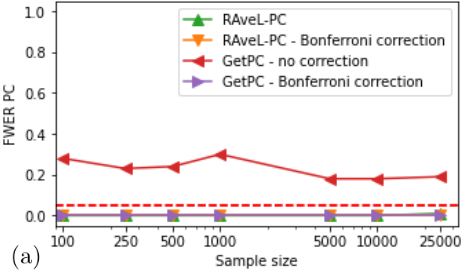
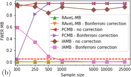
Figure 1 summarizes the estimated FWER for each sample size, and shows that RAveL-PC and RAveL-MB consistently control the FWER below the desired threshold (δ = 0.05). Moreover, in our tests the GetPC variant that exploits Bonferroni correction (see Figure 1(a)) did not return any false positive either, but in [Simionato and Vandin, 2023] we show that such configuration does not provide any guarantee on the FWER of their results. Such asymmetry is evident in Figure 1(b), in which PCMB variant with Bonferroni correction failed to bound the FWER below δ despite the results provided by GetPC did not contain any false discovery. Notably, RAveL-MB and its variant are the only algorithms with FWER guarantees for the MB discovery task. We finally analyzed the percentage of false negatives (i.e., elements that should have been returned in output but did not) for our algorithms, that are the only viable solution when the number of variables is high. Such analyses showed that the percentage of false negatives decreases for high sample sizes (25000 samples), but a simple modification of the test statistic (to be described in the full version) lowers such data requirement to just 100 samples.

Real-world data. We also run our algorithms on the Boston housing dataset [Harrison Jr and Rubinfeld, 1978] with the aim of understanding which of the variables describing Boston suburbs were related to the median price of homes in that specific area. Due to the small number of observations and variables, we ran only the variants of RAveL-PC and RAveL-MB with Bonferroni correction. Both algorithms returned in output two variables, one measuring the income of the suburb residents and a second related to the number of rooms per house. Both discoveries are sound with prior knowledge of the housing market, since rooms are a common indicator for the price of a house, and considering two identical houses, the one in the wealthier neighborhood is usually more expensive.

Acknowledgements

This work is supported, in part, by the Italian Ministry of Education, University and Research (MIUR), under PRIN Project n. 20174LF3T8 "AHeAD" (efficient Algorithms for HArnessing networked Data) and the initiative "Departments of Excellence" (Law 232/2016), and by University of Padova under project "SID 2020: RATED-X".