
Attractor-based Closed List Search: Sparsifying the Closed List for Efficient Memory-Constrained Planning
Proceedings of the Thirty-Fourth International Joint Conference on Artificial Intelligence. Main Track. Pages 9031-9038.
https://doi.org/10.24963/ijcai.2025/1004
Keywords
- Search: S: Heuristic search
Abstract
Best-first search algorithms such as A* and Weighted A* are widely used tools. However, their high memory requirements often make them impractical for memory-constrained applications, such as on-board planning for interplanetary rovers, drones, and embedded systems. One popular strategy among memory-efficient approaches developed to address this challenge is to eliminate or sparsify the Closed list, a structure that tracks states explored by the search. However, such methods often incur substantial overhead in runtime, requiring recursive searches for solution reconstruction. In this work, we propose Attractor-based Closed List Search (ACLS), a novel framework that sparsely represents the Closed list using a small subset of states, termed attractors. ACLS intelligently identifies attractor states in a way that enables efficient solution reconstruction while preserving theoretical guarantees on the quality of the solution. Furthermore, we also introduce a lazy variant, Lazy-ACLS, which defers the computation of attractor states until necessary, substantially improving planning speed. We demonstrate the efficacy of ACLS used in conjunction with A*, Weighted A*, and Dijkstra’s searches across multiple domains including 2D and 3D navigation, Sliding Tiles, and Towers of Hanoi. Our experimental results demonstrate that ACLS significantly reduces memory usage, maintaining only 9% of the states typically stored in a Closed list, while achieving comparable planning times and outperforming state-of-the-art approaches. Source code can be found at github.com/alvin-ruihua-zou/ACLS.
- [Bu and Korf, 2019] Zhaoxing Bu and Richard E Korf. A*+ ida*: A simple hybrid search algorithm. In IJCAI, pages 1206-1212, 2019. IJCAI
- [Chakrabarti et al., 1989] P.P. Chakrabarti, S. Ghose, A. Acharya, and S.C. de Sarkar. Heuristic search in restricted memory. Artificial Intelligence, 41(2):197-221, 1989.
- [Dijkstra, 1959] E. W. Dijkstra. A note on two problems in connexion with graphs. Numer. Math., 1(1):269-271, De- cember 1959.
- [Edelkamp et al., 2004] Stefan Edelkamp, Shahid Jabbar, and Stefan Schrödl. External a. In Annual Conference on Artificial Intelligence, pages 226-240. Springer, 2004.
- [Goldenberg et al., 2014] Meir Goldenberg, Ariel Felner, Roni Stern, Guni Sharon, Nathan Sturtevant, Robert C Holte, and Jonathan Schaeffer. Enhanced partial expansion a. Journal of Artificial Intelligence Research, 50:141-187, 2014.
- [Hart et al., 1968] Peter E Hart, Nils J Nilsson, and Bertram Raphael. A formal basis for the heuristic determination of minimum cost paths. IEEE transactions on Systems Sci- ence and Cybernetics, 4(2):100-107, 1968.
- [Ikeda and Imai, 1999] Takahiro Ikeda and Hiroshi Imai. En- hanced a algorithms for multiple alignments: optimal alignments for several sequences and k-opt approximate alignments for large cases. Theoretical Computer Science, 210(2):341-374, 1999.
- [Islam et al., 2019] Fahad Islam, Oren Salzman, and Maxim Likhachev. Provable indefinite-horizon real-time planning for repetitive tasks. In Proceedings of the International Conference on Automated Planning and Scheduling, vol- ume 29, pages 716-724, 2019.
- [Korf and Schultze, 2005] Richard E Korf and Peter Schultze. Large-scale parallel breadth-first search. In AAAI, volume 5, pages 1380-1385, 2005.
- [Korf et al., 2005] Richard E Korf, Weixiong Zhang, Ignacio Thayer, and Heath Hohwald. Frontier search. Journal of the ACM (JACM), 52(5):715-748, 2005.
- [Korf, 1985] Richard E Korf. Depth-first iterative- deepening: An optimal admissible tree search. Artificial intelligence, 27(1):97-109, 1985.
- [Korf, 1993] Richard E Korf. Linear-space best-first search. Artificial intelligence, 62(1):41-78, 1993.
- [Korf, 2004] Richard E Korf. Best-first frontier search with delayed duplicate detection. In AAAI, volume 4, pages 650-657, 2004.
- [Lovinger and Zhang, 2017] Justin Lovinger and Xiaoqin Zhang. Enhanced simplified memory-bounded a star (sma*+). In Christoph Benzmüller, Christine Lisetti, and Martin Theobald, editors, GCAI 2017. 3rd Global Confer- ence on Artificial Intelligence, volume 50 of EPiC Series in Computing, pages 202-212. EasyChair, 2017.
- [Pohl, 1970] Ira Pohl. Heuristic search viewed as path find- ing in a graph. Artificial intelligence, 1(3-4):193-204, 1970.
- [Reinefeld and Marsland, 1994] Alexander Reinefeld and T. Anthony Marsland. Enhanced iterative-deepening search. IEEE Transactions on Pattern Analysis and Ma- chine Intelligence, 16(7):701-710, 1994.
- [Romein et al., 1999] John W Romein, Aske Plaat, Henri E Bal, and Jonathan Schaeffer. Transposition table driven work scheduling in distributed search. In AAAI/IAAI, pages 725-731, 1999.
- [Russell, 1992] Stuart Russell. Efficient memory-bounded search methods. In Proceedings of the 10th European Conference on Artificial Intelligence, ECAI '92, page 1-5, USA, 1992.
- [Sturtevant, 2012] N. Sturtevant. Benchmarks for grid-based pathfinding. Transactions on Computational Intelligence and AI in Games, 4(2):144 -148, 2012.
- [Yoshizumi et al., 2000] Takayuki Yoshizumi, Teruhisa Miura, and Toru Ishida. A* with partial expansion for large branching factor problems. In AAAI/IAAI, pages 923-929, 2000.
- [Zhou and Hansen, 2002] Rong Zhou and Eric Hansen. Memory-bounded a* graph search. pages 203-209, 01 2002.
- [Zhou and Hansen, 2003] Rong Zhou and Eric A Hansen. Sparse-memory graph search. In IJCAI, pages 1259-1268, 2003. IJCAI
References were extracted automatically from the PDF and may contain errors.
Full text extracted automatically from the PDF; figures, tables and equations may differ. The PDF is the version of record.
1 Introduction
Best-first search algorithms have long been a cornerstone of planning systems, valued for their strong theoretical guarantees and ability to solve diverse planning problems. However, achieving these guarantees often requires significant computational and memory resources, particularly in large and complex search spaces. Over the past few decades, substantial progress has been made in improving the runtime efficiency of these algorithms. However, less attention has been given to optimizing memory utilization, a critical consideration in resource-constrained environments such as embedded systems, interplanetary rovers, and drones. In such scenarios, the high memory footprint of these algorithms can become a critical bottleneck.
The Open and Closed lists are data structures central to the operation of many widely used best-first search algorithms (including A*, Weighted A*, and Dijkstra's) [Dijkstra, 1959; Hart et al., 1968; Pohl, 1970]. The Open list maintains the search frontier by prioritizing states for expansion based on their heuristic evaluation, processing the most promising ones first. The Closed list, on the other hand, serves two critical purposes. First, it prevents the algorithm from re-expanding states that have already been expanded, thereby avoiding redundant work. Second, it facilitates solution reconstruction. Upon reaching the goal state, the solution path from the start to goal must be traced. This is achieved through backtracking, leveraging the parent pointers stored within the states. Together, these lists ensure both the efficiency and correctness of the search process. However, they are also the primary contributors to the high memory footprint of these algorithms.
Over the years, various approaches have been developed to improve the memory efficiency of best-first search algorithms [Korf, 1993; Reinefeld and Marsland, 1994; Edelkamp et al., 2004; Lovinger and Zhang, 2017; Bu and Korf, 2019], as discussed in Section 2. A particularly effective strategy involves sparsifying (reducing the size of) or completely eliminating the Closed list [Zhou and Hansen, 2003; Korf et al., 2005]. While this significantly reduces memory usage, it comes at the cost of increased computation time. Techniques have been developed to mitigate state re-expansion in the absence of the Closed list [Zhou and Hansen, 2003; Korf et al., 2005]. However, eliminating or naively sparsifying the Closed list compromises the ability to quickly backtrack from the goal state to reconstruct the solution path. Instead, it requires a series of recursive searches, resulting in much longer planning times.
To this extent, in this manuscript we propose Attractorbased Closed List Search (ACLS) framework. As opposed to completely eliminating the Closed list, our framework intelligently identifies and maintains a small subset of states, termed attractors, which enables the reconstruction of the solution without performing recursive searches. The key idea is that a complete path between the start and goal can be reconstructed from a sparse set of intermediate states guided by a heuristic function. For example, in Figure 1, a 10-state path from the start to the goal can be represented using just three states (sgoal, sstart, and sattractor) and the Euclidean heuristic function. By greedily selecting predecessors based on heuristic minimization, i.e., minimizing the Euclidean heuristic function with respect to the next attractor state (either sattractor if on the right segment or sstart if on the left segment), which we refer to as Attractor-based greedy tracing, the path can be reconstructed efficiently from the goal back to the start. This approach reduces the number of stored states in the Closed list to only the necessary intermediates, drastically cutting memory usage while still supporting solution reconstruction. To ensure that all relevant paths are represented, ACLS evaluates each state to determine whether it should be stored as an attractor. However, a naive implementation of this process could lead to excessive computational overhead. To mitigate this, we also introduce a lazy variant of the framework, Lazy-ACLS (LACLS), which postpones these evaluations until necessary, accelerating the planning process.
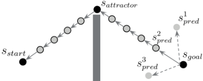
ACLS and LACLS are generic frameworks compatible with various optimal and bounded-suboptimal search algorithms. In this manuscript, we evaluate their performance with A*, Weighted A*, and Dijkstra's across diverse domains, including 2D and 3D navigation, Sliding Tiles, and Towers of Hanoi. Our results demonstrate the ability of our framework to significantly reduce memory usage, retaining only 9% of the states typically stored in a Closed list, while still maintaining competitive planning times.
2 RelatedWork
Over the years, two broad classes of ideas have been explored to reduce the memory utilization of best-first search algorithms. The first class focuses on reducing the size of the Open list. Techniques include pruning states with high f-values [Ikeda and Imai, 1999], partially expanding states to prioritize the most promising successors [Yoshizumi et al., 2000; Goldenberg et al., 2014], and pruning the least promising states and then regenerating them if no solution is found [Chakrabarti et al., 1989; Russell, 1992; Zhou and Hansen, 2002; Lovinger and Zhang, 2017]. While effective, these strategies are tangential to our work which aims to sparsify the Closed list.
The second major class of techniques, which we closely identify with, focuses on reducing the size of the Closed list. Frontier Search [Korf et al., 2005] eliminates the Closed list by maintaining a set of action operators for each state. These operators enable the search to avoid re-expanding states in the absence of the Closed list. However, by removing the Closed list, solution reconstruction now requires a series of recursive searches. Each search identifies a midpoint on the optimal path, and Frontier Search is recursively called to find a path from the start to the midpoint and from the midpoint to the goal. A similar method, Sparse Memory Graph Search
(SMGS) [Zhou and Hansen, 2003], retains only a portion of the Closed list by dividing it into a kernel and a boundary. The boundary contains expanded states that have at least one immediate successor in the search frontier (i.e., Open list), while the kernel contains the rest of the states. Since the kernel states do not impact the optimal path to states in the Open list, they are deleted when the size of the Closed list reaches some predefined threshold. To reconstruct the solution, SMGS keeps track of relay states, which, like the midpoints in Frontier Search, divide the search into smaller subproblems. While effective in reducing memory, both approaches significantly increase time complexity. Empirical comparisons with Frontier Search and SMGS are examined in Section 5.
Apart from the two broad approaches mentioned above, depth-first approaches have also been developed, including Recursive Best-First Search [Korf, 1993] and IterativeDeepening-A* [Korf, 1985], solving problems in linear space by performing a series of depth-first searches with increasing depth. However, these methods cannot detect different paths that lead to the same state, resulting in duplicate search efforts. Enhancements such as using transposition tables [Reinefeld and Marsland, 1994; Romein et al., 1999] or combing IDA* with other algorithms [Bu and Korf, 2019] reduces duplicate search efforts, but the runtime still remains a bottleneck.
Efforts have also been made to address high memory consumption by utilizing external memory. These include storing the Open and Closed lists on disk [Korf, 2004; Edelkamp et al., 2004; Korf and Schultze, 2005], which extends memory capacity but incurs additional I/O overhead. Finally, our work draws inspiration from the concept of attractors introduced by [Islam et al., 2019], which were used for offline computation to allow the planner to compute solutions online within a predefined time bound. However, our focus is diametrically different, it is to utilize attractors to sparsely represent the Closed list.
3 Terminologies and Preliminary
Let S denote the search space and let s ∈ S represent a state within this space. The set of successor states directly reachable from s is denoted as Succ(s), while the set of predecessor states that directly lead to s is represented as Pred(s). The cost of transitioning from a state s to a successor state s′ is defined by the cost function c(s, s′ ). Given a start state sstart ∈ S and a goal state sgoal ∈ S, the optimal solution path π∗ = {sstart, s1, s2, ...sgoal} is a sequence of states such that each consecutive pair of states are directly connected, i.e., si+1 ∈ Succ(si), and the total path cost c(π∗ ), defined by the summation of the transition costs c(π∗ ) = ∑i∈len(π∗ ) c(si, si+1), is minimized.
In undirected graphs, successors and predecessors are identical for all states (Succ(s) = Pred(s), ∀s ∈ S). Although in this manuscript the ACLS framework is illustrated using undirected graphs, it applies to directed graphs as well.
Typical best-first search algorithms maintain two lists, the Open list and the Closed list. The Closed list contains states that have been expanded, and the Open list contains states that have been generated but not yet expanded. For a state s, let g(s) be the cost from the start state sstart to s, and h(s) be the estimated cost from s to the goal state sgoal, given by a consistent heuristic function (h is consistent if, for all states s and s′ , h(s) ≤ c(s, s′ ) + h(s′ )). A backpointer, s.parent, represents the best parent leading to s. The states in the Open list are ordered for expansion based on a priority function (e.g., g(s) + w ∗ h(s),w ≥ 0). During the expansion process, all successors of the current state are generated. Those that have not been previously expanded are added to the Open list, while the expanded state itself is moved to the Closed list.
[Korf et al., 2005] introduced the idea of action operators to circumvent the problem of re-expanding states in the absence of a Closed list. Each operator corresponds to an action, and when a state s is expanded, all predecessors s′ ∈ Pred(s) mark their operator associated with the action of generating s as used. This ensures that when a predecessor s′ is expanded, the action that regenerates s is excluded. However, operators do not encode any information that can help with solution reconstruction. Hence, in our framework we adopt the idea of operators to prevent re-expansions, and develop the idea of attractors to enable efficient solution reconstruction. It should be noted that our framework can also be combined with other techniques that prevent state re-expansions (e.g., SMGS).
Since our framework relies on the concept of greedy tracing, we begin by defining the notions of a greedy predecessor and greedy tracing, inspired by [Islam et al., 2019], before detailing how the algorithm operates.
Definition 1. Let s be some state and s′ its predecessor. s′ is a greedy predecessor of s with respect to some nonnegative function p(s), i.e., p(s) ≥ 0∀s ∈ S, if it has the minimal p-value with respect to all predecessors of s, i.e., s′ = argmins′′∈Pred(s)p(s′′ ).
Note that for a given p and a deterministic tiebreaking rule, every state with a non-zero number of incoming edges has a unique greedy predecessor. In our framework, a predefined action order induces an order over parent states; ties are broken in favor of the earliest parent in this order.
Definition 2. Given such a function p and some deterministic tiebreaking rule, an algorithm is said to greedily trace with respect to p if, for any state, it iteratively identifies and returns its greedy predecessor according to p, terminating when reaching a state with p(s) = 0.
Note that we have defined greedy tracing in the backward direction, i.e., picking the best predecessor (instead of the successor), the reason for which will become clearer once we elucidate how we utilize it. We assume that the framework has access to some deterministic tiebreaking and a non-negative heuristic function, hdist : S × S → R, s.t., hdist(s, s′ ) ≥ 0 ∀ s, s′ ∈ S, which estimates the distance between any two states in S. The heuristic function satisfies the property hdist(s, s) = 0, i.e., the heuristic estimate from a state to itself is 0. Given such a heuristic function hdist, an algorithm is said to greedily trace toward a target state s ∈ S if we trace with respect to a function p, where p is parameterized by s and is equal to hdist(s, s′ ), ∀ s′ ∈ S.
4 Methodology
In typical best-first search algorithms, all expanded states are stored in the Closed list. Upon expanding the goal state, the solution path is reconstructed by starting at the goal and iteratively moving to the best parent by either following backpointers if they were maintained during the search or computing a parent state whose g-value plus the cost of the transition is minimal among all parents. Either of these options relies on having access to the entire Closed list. Our key insight is to replace the Closed list with a sparse set of states called attractors, such that the reconstruction of the solution becomes a series of greedy traces with respect to the attractors, with every greedy trace recovering a segment of the optimal path.
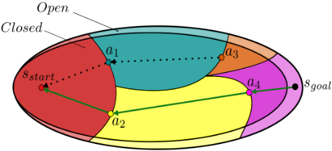
The ACLS framework is structured similarly to a typical best-first search, with one key difference: instead ofmaintaining a Closed list, the algorithm maintains a set of attractors, denoted as Attractors. The main algorithm is presented in Algorithm 1 with the procedures for creating and deleting attractors detailed in UPDATEATTRACTOR and TIEBREAKATTRACTOR. Solution reconstruction is outlined in the RECONSTRUCTPATH procedure. To reiterate, ACLS is a generic framework, and the ideas employed by it can be integrated with a number of search algorithms.
ACLS
Every state generated by the search is assigned an attractor state, which is always one of the previously expanded states. An attractor a is assigned to a state s, if i) a greedy trace from s towards a recovers the current best path from a to s, and ii) this recovered path is a segment of the current best path from the start state sstart to s. Every state's best parent qualifies to be its attractor. However, our objective is to assign each attractor to many states, enabling path reconstruction while reducing the number of attractors stored in memory.
Every attractor state except the start state has its own parent attractor. Since attractors are expanded states and the search ensures the discovery of (bounded sub-)optimal paths to all expanded states, the presence of a parent attractor for every attractor ensures that the (bounded sub-)optimal path from the start state to any attractor can be reconstructed through successive greedy traces from the attractor to its parent attractor and onward. This hierarchical structure allows for the reconstruction of the current best path to any state in the Open list. This ensures that when the goal state is expanded the (bounded sub-)optimal solution can be reconstructed.
This methodical creation and assignment of attractor states ensure that at any point during the search, both the Closed and Open lists can be conceptually decomposed into subregions, each associated with an attractor as illustrated in Figure 2. Greedy tracing from a closed (or open) state to its assigned attractor, followed by successive traces from the attractor to its parent attractor, allows for the reconstruction of the optimal (or current best) path to that state. Maintaining these attractors is enough to recover all relevant solutions, and all other expanded states can be deleted.
Algorithm 1 ATTRACTOR-BASED CLOSED LIST SEARCH
Input: sstart, sgoal ∈ S Output: solution path π 1: procedure ACLS(sstart, sgoal) 2: INSERT sstart in Open with f(sstart) 3: INSERT sstart in Attractors with parent ∅ 4: while Open ̸= ∅ do 5: POP s with the smallest f-value from Open 6: if s = sgoal then 7: return RECONSTRUCTPATH(sstart, sgoal) 8: end if 9: for s′ ∈ Succ(s) do 10: if s.operator(s′ ) = used then 11: continue 12: end if 13: s′ .operator(s) = used 14: if g(s′ ) > g(s) + c(s, s′ ) then 15: g(s′ ) = g(s) + c(s, s′ ) 16: UPDATEATTRACTOR(s, s′ ) 17: else if g(s′ ) = g(s) + c(s, s′ ) then 18: TIEBREAKATTRACTOR(s, s′ ) 19: end if 20: if s′ /∈ Open then 21: INSERT s′ in Open with f(s′ ) 22: end if 23: end for 24: DELETE s 25: DELETE all a ∈ Attractors that are unassigned 26: end while 27: end procedure 28: procedure UPDATEATTRACTOR(s, s′ ) 29: s′′min ← argmins′′ ∈P red(s′ ) hdist(s′′ , s.attractor) 30: s′ .attractor ← s 31: if s′′min = s then 32: s′ .attractor ← s.attractor 33: else if s not in Attractors then 34: INSERT s in Attractors with parent s.attractor 35: end if 36: end procedure 37: procedure TIEBREAKATTRACTOR(s, s′ ) 38: s′′min ← argmins′′ ∈P red(s′ ) hdist(s′′ , s.attractor) 39: if s′′min = s then 40: if hdist(s′ , s.attr) > hdist(s′ , s′ .attr) then 41: s′ .attractor ← s.attractor 42: end if 43: end if 44: end procedureHence, the high level idea is that during every expansion we determine if the state s that is being expanded is required to reconstruct the current best path to any of its successors s′ . If it is, we store s as an attractor (line 34, Alg. 1). If not, we delete the state (line 24, Alg. 1).
When expanding s, if a better path to one of its successors s′ is discovered, we must be able to reconstruct this new path to s′ . To minimize the number of attractors saved, we attempt to assign s′ the same attractor as s. For s′ to inherit s's attractor, it is necessary that s′ 's greedy tracing through this attrac-
Algorithm 2 RECONSTRUCTPATH
Input: sstart, sgoal ∈ S Output: solution path π Global: Attractors, hdist 1: scurr ← sgoal 2: acurr ← sgoal.attractor 3: π ← scurr 4: while scurr ̸= sstart do 5: while scurr ̸= acurr do 6: scurr ← argmins′ ∈P red(scurr) hdist(s′ , acurr) 7: π ← π ∪ {scurr} 8: end while 9: scurr ← acurr 10: acurr ← acurr.parent 11: end while 12: return Reverse(π)tor leads to s. If this condition is met, s can be deleted without affecting the path reconstruction. If this condition is not met, then s itself is assigned as the attractor for s′ , in which case it is saved with its parent attractor set to s.attractor (line 34, Alg. 1). By assigning s′ 's attractor in this way, the best path to s′ is always recoverable.
Attractor maintenance relies on a data structure called Attractors. This structure maintains the list of attractors, along with their parent attractor and a counter representing the number of states assigned to each attractor (line 34, Alg. 1). These states include both those in the Open list and those within the Attractors structure itself. The counter is dynamically updated as states are newly assigned to an attractor, reassigned to a different attractor, or removed from the Open list. If an attractor is no longer assigned to any state (counter is zero), it is deleted from the Attractors structure (line 25, Alg. 1).
Tiebreaking
When multiple paths of the same cost lead to a state s, we tiebreak by selecting the path that assigns an attractor farthest from s. Here, "farther away" is quantified as the attractor with a higher hdist value relative to s. For example, consider two parents s′ and s′′ , both sharing the same attractor t. If s′ is the greedy predecessor of s based on t (due to deterministic tiebreaking), but s′′ was expanded first, s′′ might be unnecessarily added to the Attractors structure and assigned as s's attractor instead of t. To prevent such scenarios, we tiebreak by favoring the path with the attractor that is farther away (line 40, Alg. 1), such that t will be assigned as s's attractor once s′ is expanded. Alternatively, it is possible to bypass the tiebreaking routine altogether at the expense of saving more attractors. The empirical impact of this tiebreaking strategy is analyzed in Section 5.5.
Lazy-ACLS
The major computational overhead in maintaining attractors is the routine required for calculating the greedy predecessor of a successor state s′ whenever the same or better cost path to it is found during the expansion of a state s. This process involves enumerating all predecessors of s′ and verifying whether s has the smallest hdist value with respect to s.attractor among them (UPDATEATTRACTOR). Repeating this evaluation for every generated state can be computationally expensive, particularly in high-branching scenarios. To mitigate this, we propose a lazy evaluation approach that defers these computations until s′ is expanded (Alg. 3).
The key insight is that, at the time of expanding a state s, its attractor is either its best parent (bp) or the attractor of its best parent (bp attractor). Rather than calculating and assigning the attractor each time a better path to s is found, we store the current best parent and its attractor for all generated states, updated as better paths are discovered. When s is finally expanded, we use the stored parent and its attractor to determine s's attractor (line 6, Alg. 3). Although this approach incurs a minor additional cost in terms of memory, it significantly reduces the computational burden by postponing attractor calculations until expansion.
In experiments, we tested two tiebreaking strategies for handling same-cost paths to a state s. The first strategy heuristically selects the parent with the farthest attractor, despite uncertainty over whether the parent (bp) or its attractor (bp attractor) will ultimately be assigned to s. The second strategy stores all parents (and their attractors) associated with same-cost paths. At the time of s's expansion, the attractor corresponding to each parent is computed sequentially, and the first attractor that matches s's greedy predecessor to bp is assigned. Both strategies were implemented, with the first being more effective. Ablation studies in Section 5.5 examine the impact of these strategies.
Theoretical Properties
Theorem 1. When ACLS is used with the priority function f = g + h, where h is a consistent heuristic function (i.e., ACLS with A*), the path recovered by recursively performing greedy traces from state sgoal at the time of its expansion is guaranteed to be optimal.
Proof Sketch. We prove this by induction.
Base Case: The optimal path to s′ , a successor of sstart, is recoverable at the time of its expansion. As sstart does not have a parent attractor it will be assigned as s′ 's attractor, thus guaranteeing the recovery of the optimal path to s′ .
Inductive Step: Let s ∈ Pred(s′ ) be the sole best parent of s′ . If a recursive greedy trace from s at the time of its expansion recovers the optimal path from sstart to s, we must show that a recursive greedy trace from s′ at the time of its expansion is also guaranteed to recover the optimal solution.
If s is the best parent of s′ , then it is guaranteed to be expanded before s′ (since h(s) is consistent). At the time of its expansion the framework is guaranteed to enter the UPDATEATTRACTOR(s, s′ ) routine. Here, the framework verifies if s is the greedy predecessor of s′ with respect to s.attractor. If it is, then recursively greedy tracing from s′ to s.attractor and from s.attractor to its parent attractor is guaranteed to return the optimal solution to s′ , as a recursive greedy trace from s to s.attractor recovers the optimal solution to s. If not, then s is assigned as the attractor to s′ with its parent attractor being s.attractor. In which case, again, recursively greedy tracing from s′ recovers the optimal solution. A similar case can be made for when there are multiple best parents, in which case the search would enter the TIEBREAKATTRACTOR(s, s′ ) routine.
A proof identical to this exists for when the framework is integrated with a bounded suboptimal search, where the recursive greedy traces from sgoal recover the bounded sub-
Algorithm 3 Lazy-ACLS
Input: sstart, sgoal ∈ S Output: solution path π 1: procedure LACLS(sstart, sgoal) 2: INSERT sstart in Open with f(sstart) 3: INSERT sstart in Attractors with parent ∅ 4: while OPEN ̸= ∅ do 5: POP s with the smallest f-value from Open 6: UPDATEATTRACTOR(s.bp, s) 7: if s = sgoal then 8: return RECONSTRUCTPATH(sstart, sgoal) 9: end if 10: for s′ ∈ Succ(s) do 11: if s.operator(s′ ) = used then 12: continue 13: end if 14: s′ .operator(s) = used 15: if g(s′ ) > g(s) + c(s, s′ ) then 16: g(s′ ) = g(s) + c(s, s′ ) 17: s′ .bp = s; s′ .bp attractor = s.attractor 18: else if g(s′ ) = g(s) + c(s, s′ ) then 19: TIEBREAKATTRACTORLAZY(s, s′ ) 20: end if 21: if s′ /∈ OPEN then 22: INSERT s′ in Open with f(s′ ) 23: end if 24: end for 25: end while 26: end procedure 27: procedure TIEBREAKATTRACTORLAZY(s, s′ ) 28: if hdist(s′ .bp, s′ .bp attractor) < hdist(s, s.attractor) then 29: s′ .bp ← s 30: s′ .bp attractor ← s.bp attractor 31: end if 32: end procedureoptimal path to sgoal. It is important to note that while the heuristic function h must be consistent to ensure optimality, the function hdist used for greedy tracing toward attractors need not be.
5 Experimental Results
The performance of our framework is presented on four different domains: 2D and 3D grid world navigation, Sliding Tiles and Towers of Hanoi. We compare the performance of ACLS and Lazy-ACLS (LACLS) against memory-efficient baselines that focus on sparsifying/eliminating the Closed list: Frontier Search with A* (FA*) and SMGS (described in Section 2). All planners utilize a priority function of f = g + w ∗ h, with w = 1, unless explicitly mentioned otherwise. For each problem, the SMGS threshold for pruning the Closed list was set to 10% the size of A*'s Closed list at termination.
5.1 2DNavigation
Table 2 presents the results averaged over 2,500 problems evaluated across five maps from the Moving AI 2D benchmark [Sturtevant, 2012] (random512-10-0, maze512-1-0, brc202d, den012d, orz800d). A 4-connected grid action set was used, with the Manhattan distance serving as both the search heuristic and the attractor distance function hdist.
| Weight | A* | ACLS | LACLS | FA* | SMGS | |||||
|---|---|---|---|---|---|---|---|---|---|---|
| Runtime (ms) | Closed states | Runtime (ms) | Closed states | Runtime (ms) | Closed states | Runtime (ms) | Closed states | Runtime (ms) | Closed states | |
| 0 (Dijkstra's) | 65.6 | 59,955 | 95.0 | 306 | 83.0 | 291 | 368.2 | - | 2,299 | 6,000 |
| 1 (A*) | 18.0 | 20,340 | 26.0 | 631 | 23.0 | 353 | 101.0 | - | 3,192 | 2,533 |
| 5 (WA*) | 7.5 | 8,431 | 10.5 | 432 | 10.7 | 218 | 61.2 | - | 353.1 | 1,071 |
| 10 (WA*) | 6.0 | 6,575 | 8.3 | 396 | 8.6 | 180 | 49.8 | - | 359.4 | 883 |
| Planner | Plan Time (ms) | Closed states | Open Mem. (bytes) | Closed Mem. (bytes) | Total Mem. (bytes) |
|---|---|---|---|---|---|
| A* | 18 | 20,340 | 20,115 | 325,440 | 345,555 |
| ACLS | 26 | 631 | 17,601 | 10,102 | 27,703 |
| LACLS | 23 | 353 | 22,630 | 5,850 | 28,480 |
| FA* | 101 | - | 20,115 | - | 20,115 |
| SMGS | 3,192 | 2,533 | 17,601 | 50,669 | 68,270 |
The results highlight the effectiveness of ACLS and LACLS in significantly sparsifying the Closed list while maintaining competitive runtimes. LACLS achieves a runtime only 1.3 times slower than A*, while reducing the size of the Closed list by a factor of 58. ACLS performs similarly, with a 1.4 times slowdown and a 32-fold reduction in the Closed list size. As expected, LACLS improves planning speed by postponing attractor computation to the state expansion phase. This not only enhances efficiency but also results in fewer attractors, by eliminating attractors created by states that were generated but never expanded in ACLS. The strong planning times achieved by our frameworks contrast with those of FA* and SMGS. While FA* achieves greater memory savings by completely eliminating the Closed list, it is significantly slower, taking 5.6 times the runtime of A*. SMGS has the worst overall performance, running 177.3 times slower while reducing the Closed list by a factor of 8.
| Planner | Plan Time (ms) | Closed states | Open Mem. (Kb) | Closed Mem. (Kb) | Total Mem. (Kb) |
|---|---|---|---|---|---|
| A* | 523.7 | 219,464 | 513.3 | 3,511.4 | 4,024.7 |
| ACLS | 653.3 | 7,202 | 449.1 | 115.2 | 564.4 |
| LACLS | 540.8 | 3,613 | 577.4 | 57.8 | 635.2 |
| FA* | 949.6 | - | 513.3 | - | 513.3 |
To provide a comprehensive view of memory efficiency, we explicitly report the memory consumption of each planner, reflecting the data required to maintain the Open and Closed lists. As expected, LACLS consumes more memory for its Open list than ACLS, even though both maintain the same number of Open states. This additional memory is due to the bookkeeping needed to determine attractors at expansion, which we optimized to incur only 8 additional bytes per Open state. In this domain, the Closed list is significantly larger than the Open list, making its reduction critical for memory savings. By dramatically reducing the size of the Closed list, ACLS (and LACLS) achieves up to 12.5x (and 12.1x) memory savings compared to A*, similar to the savings achieved by FA* (17.2x).
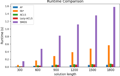
We also present the impact of path length on runtime in Fig. 3. As path length increases, planning times rise for FA* and SMGS compared to A*, as they require more recursive searches to reconstruct the path. The runtime of FA* compared to A* increases from 5.7 to 10.2, while ACLS and LACLS remain relatively stable (around 1.5 and 1.3).
To understand the impact of our framework when used with Dijkstra, A*, and Weight A* (WA*), we altered the heuristic weight w in the priority function and studied the performance of the planners (Table 1). We observe that as w increases, the memory savings achieved decreases. LACLS reduces the size of the Closed list by a factor of 206 when w = 0, but goes down to 36.5 for w = 10.
5.2 3DNavigation
Table 3 summarizes the results averaged over 3,000 problems evaluated on three maps from the Moving AI 3D benchmark [Sturtevant, 2012] (A1, BA1, DC3) A 6-connected grid action set was employed, with Manhattan distance used as both the search heuristic and the attractor distance function hdist. The trends observed are consistent with those in 2D navigation. LACLS achieves a runtime nearly identical to A* while reducing the Closed list size by a factor of 61, demonstrating its potential to significantly reduce memory usage with minimal runtime overhead. FA* also performs better in this domain, exhibiting a smaller relative slowdown compared to its performance in the 2D case. The algorithms demonstrate a similar reduction in memory footprint, with LACLS reducing memory usage (in comparison to A*) by a factor of 6.3, while FA* achieves a reduction of 7.8. SMGS, tested with a timeout of 30x the time of A*, exhibited a poor success rate of 7%, and therefore its results are omitted from the table.
| Path | A* | ACLS | LACLS | FA* | ||||
|---|---|---|---|---|---|---|---|---|
| Length | Runtime (ms) | Closed states | Runtime (ms) | Closed states | Runtime (ms) | Closed states | Runtime (ms) | Closed states |
| 25 | 27.8 | 1,594 | 39.7 | 437 | 33.4 | 234 | 66.0 | - |
| 27 | 35.1 | 2,042 | 55.2 | 550 | 43.8 | 294 | 85.9 | - |
| 29 | 128.9 | 7,427 | 182.4 | 2,037 | 151.6 | 1,086 | 295.0 | - |
| 31 | 131.8 | 7,509 | 183.3 | 2,083 | 159.5 | 1,128 | 299.9 | - |
| 33 | 539.4 | 30,927 | 743.4 | 8,295 | 640.8 | 4,467 | 1,192.8 | - |
| 35 | 445.3 | 26,065 | 612.4 | 6,926 | 541.3 | 3,793 | 1,000.8 | - |
| Discs | A* | ACLS | LACLS | FA* | SMGS | |||||
|---|---|---|---|---|---|---|---|---|---|---|
| Runtime (ms) | Closed states | Runtime (ms) | Closed states | Runtime (ms) | Closed states | Runtime (ms) | Closed states | Runtime (ms) | Closed states | |
| 4 | 0.312 | 49 | 0.905 | 11 | 0.634 | 12 | 1.7 | - | 8.74 | 14 |
| 6 | 2.71 | 518 | 5.58 | 92 | 4.2 | 88 | 14.1 | - | 51.8 | 57 |
| 7 | 9.16 | 1,715 | 17.8 | 298 | 13.5 | 254 | 46.3 | - | 173 | 175 |
| 9 | 93.7 | 17,348 | 173 | 3,009 | 131 | 2,280 | 454 | - | 1,720 | 1,741 |
| 10 | 282 | 54,127 | 519 | 9,383 | 414 | 6,957 | 1,429 | - | 5,752 | 5,418 |
| 12 | 2,767 | 508,038 | 4,961 | 87,887 | 3,804 | 64,351 | 14,128 | - | 90,074 | 50,808 |
| 13 | 8,889 | 1,545,697 | 15,209 | 267,325 | 11,650 | 194,627 | 43,753 | - | 432,193 | 154,573 |
| 14 | 27,382 | 4,679,464 | 45,937 | 809,140 | 35,651 | 587,446 | 136,538 | - | 2,764,541 | 467,957 |
5.3 Sliding Tiles
Table 4 summarizes the results averaged over 55 random fifteen Sliding Tiles puzzles with six different solution lengths. The Manhattan distance + linear conflicts was used for the heuristic and the number of mismatched tiles was used for the attractor distance function hdist. LACLS achieves a runtime 1.2 times slower and reduces the size of the Closed list by a factor of 6.9 compared to A*, while FA* experiences a slowdown of 2.2. SMGS again performed poorly in this domain, timing out for every instance (30x time of A*). As such, its results are omitted from the table.
5.4 Towers of Hanoi
Table 5 presents the results of the planners for three pegs Towers of Hanoi with different numbers of discs, using the number of misplaced discs as the heuristic and the attractor distance function hdist. The results highlight that LACLS achieves substantial savings in planning time compared to FA*. Specifically, LACLS incurs an average slowdown of only 1.3 times and ACLS 1.7 times, while FA* has a slowdown of 5 times. In terms of memory, LACLS reduces the size of the Closed list by 8 times compared to A*, and ACLS achieves a factor of 5.8. On the other hand, SMGS experiences a considerable slowdown of 83.6 times compared to A*, with a Closed list reduction factor of 10.
5.5 Ablations
This subsection presents ablation studies analyzing the impact of two key design choices. The first study focuses on the effect of using TIEBREAKATTRACTOR in ACLS. When tiebreaking was omitted, the number of attractors stored increased drastically by 25 times while the runtime remained constant, as expected. This highlights the importance of tiebreaking. For LACLS, the impact was less pronounced, with an increase of 5 times when tiebreaking was not employed. This difference may be attributed to LACLS inherently requiring fewer attractors than ACLS.
The other study investigates different tiebreaking strategies for LACLS. One approach involved maintaining a list of parents (and their attractors) for cases where multiple paths with the same cost exist, while another only kept one parent (and attractor) by heuristically selecting the parent with a farther attractor. Both strategies produced a similar number of attractors, but the additional bookkeeping and evaluations required in the first approach resulted in a 2 times slowdown. Consequently, the heuristic-based strategy was preferred.
6 Conclusion
In this work, we introduced a general and effective framework that intelligently sparsifies the Closed list by maintaining a small subset of states, referred to as attractors. These attractors enable efficient solution path reconstruction through a series of greedy traces. Compatible with various search algorithms, the developed ACLS and LACLS frameworks significantly reduce memory requirements-retaining only 9% of the states typically stored in a Closed list-while delivering competitive planning times across diverse problem domains.
Acknowledgments
The research was supported by the National Science Foundation by grant IIS-2328671. The views and conclusions in this document are those of the authors and should not be interpreted as representing the official policies, either expressed or implied, of the sponsoring organizations, agencies, or the U.S. government.
@inproceedings{ijcai2025p1004,
  title     = {Attractor-based Closed List Search: Sparsifying the Closed List for Efficient Memory-Constrained Planning},
  author    = {Zou, Alvin and Saleem, Muhammad Suhail and Likhachev, Maxim},
  booktitle = {Proceedings of the Thirty-Fourth International Joint Conference on
               Artificial Intelligence, {IJCAI-25}},
  publisher = {International Joint Conferences on Artificial Intelligence Organization},
  editor    = {James Kwok},
  pages     = {9031--9038},
  year      = {2025},
  month     = {8},
  note      = {Main Track},
  doi       = {10.24963/ijcai.2025/1004},
  url       = {https://doi.org/10.24963/ijcai.2025/1004},
}
TY - CPAPER TI - Attractor-based Closed List Search: Sparsifying the Closed List for Efficient Memory-Constrained Planning AU - Zou, Alvin AU - Saleem, Muhammad Suhail AU - Likhachev, Maxim T2 - Proceedings of the Thirty-Fourth International Joint Conference on Artificial Intelligence, IJCAI-25 PB - International Joint Conferences on Artificial Intelligence Organization PY - 2025 SP - 9031 EP - 9038 DO - 10.24963/ijcai.2025/1004 UR - https://doi.org/10.24963/ijcai.2025/1004 ER -Copied
Machine-readable versions of this paper, for tools and AI agents:





