
LLM-enhanced Score Function Evolution for Causal Structure Learning
Proceedings of the Thirty-Fourth International Joint Conference on Artificial Intelligence. Main Track. Pages 9086-9094.
https://doi.org/10.24963/ijcai.2025/1010
Keywords
- Constraint Satisfaction and Optimization: CSO: Constraint optimization problems
- Uncertainty in AI: UAI: Causality, structural causal models and causal inference
- Uncertainty in AI: UAI: Bayesian networks
- Search: S: Evolutionary computation
Abstract
Causal structure learning (CSL) plays a pivotal role in causality and is often formulated as an optimization problem within score-and-search methods. Under the assumption of an infinite dataset and a predefined distribution, several well-established and consistent score functions have been shown to be both optimal and reliable for identifying ground-truth causal graphs. However, in practice, these idealized assumptions are often infeasible, which can result in CSL algorithms learning suboptimal structures. In this paper, we introduce L-SFE, a framework designed to automatically discover effective score functions by exploring the "score function space". L-SFE addresses this task from a bi-level optimization perspective. First, it leverages a Large Language Model (LLM) to interpret the characteristics of score functions and generate the corresponding code implementations. Next, L-SFE employs evolutionary algorithms along with carefully designed operators, to search for solutions with higher fitness. Additionally, we take the BIC as example and prove the consistency of the generated score functions. Experimental evaluations, conducted on discrete, continuous, and real datasets, demonstrate the high stability, generality and effectiveness of L-SFE.
- [Achiam et al., 2023] Josh Achiam, Steven Adler, Sandhini Agarwal, Lama Ahmad, Ilge Akkaya, Florencia Leoni Aleman, Diogo Almeida, Janko Altenschmidt, Sam Alt- man, Shyamal Anadkat, et al. Gpt-4 technical report. arXiv preprint arXiv:2303.08774, 2023.
- [Andrews et al., 2018] Bryan Andrews, Joseph Ramsey, and Gregory F Cooper. Scoring bayesian networks of mixed variables. International journal of data science and ana- lytics, 6:3-18, 2018.
- [Andrews et al., 2023] Bryan Andrews, Joseph Ramsey, Ruben Sanchez Romero, Jazmin Camchong, and Erich Kummerfeld. Fast scalable and accurate discovery of dags using the best order score search and grow shrink trees. Advances in Neural Information Processing Sys- tems, 36:63945-63956, 2023.
- [Ban et al., 2023] Taiyu Ban, Lyuzhou Chen, Derui Lyu, Xi- angyu Wang, and Huanhuan Chen. Causal structure learn- ing supervised by large language model. arXiv preprint arXiv:2311.11689, 2023.
- [Bello et al., 2022] Kevin Bello, Bryon Aragam, and Pradeep Ravikumar. Dagma: Learning dags via m-matrices and a log-determinant acyclicity characteriza- tion. Advances in Neural Information Processing Systems, 35:8226-8239, 2022.
- [Cheng et al., 2024] Debo Cheng, Jiuyong Li, Lin Liu, Jixue Liu, and Thuc Duy Le. Data-driven causal effect estima- tion based on graphical causal modelling: A survey. ACM Computing Surveys, 56(5):1-37, 2024.
- [Chickering, 1996] David Maxwell Chickering. Learning bayesian networks is np-complete. Learning from data: Artificial intelligence and statistics V, pages 121-130, 1996.
- [Chickering, 2002] David Maxwell Chickering. Learning equivalence classes of bayesian-network structures. The Journal of Machine Learning Research, 2:445-498, 2002.
- [Colombo et al., 2014] Diego Colombo, Marloes H Maathuis, et al. Order-independent constraint-based causal structure learning. J. Mach. Learn. Res., 15(1):3741-3782, 2014.
- [Constantinou et al., 2022] Anthony C Constantinou, Yang Liu, Neville K Kitson, Kiattikun Chobtham, and Zhigao Guo. Effective and efficient structure learning with prun- ing and model averaging strategies. International Journal of Approximate Reasoning, 151:292-321, 2022.
- [Constantinou et al., 2023] Anthony Constantinou, Neville K Kitson, Yang Liu, Kiattikun Chobtham, Arian Hashemzadeh Amirkhizi, Praharsh A Nanavati, Rendani Mbuvha, and Bruno Petrungaro. Open problems in causal structure learning: A case study of covid-19 in the uk. Expert Systems with Applications, 234:121069, 2023.
- [Glymour et al., 2019] Clark Glymour, Kun Zhang, and Pe- ter Spirtes. Review of causal discovery methods based on graphical models. Frontiers in genetics, 10:524, 2019.
- [Haughton, 1988] Dominique MA Haughton. On the choice of a model to fit data from an exponential family. The annals of statistics, pages 342-355, 1988.
- [Heckerman et al., 1995] David Heckerman, Dan Geiger, and David M Chickering. Learning bayesian networks: The combination of knowledge and statistical data. Ma- chine learning, 20:197-243, 1995.
- [Huang et al., 2018] Biwei Huang, Kun Zhang, Yizhu Lin, Bernhard Schölkopf, and Clark Glymour. Generalized score functions for causal discovery. In Proceedings of the 24th ACM SIGKDD international conference on knowl- edge discovery & data mining, pages 1551-1560, 2018.
- [Jiralerspong et al., 2024] Thomas Jiralerspong, Xiaoyin Chen, Yash More, Vedant Shah, and Yoshua Bengio. Efficient causal graph discovery using large language models. In ICLR 2024 Workshop: How Far Are We From AGI, 2024.
- [Khatibi et al., 2024] Elahe Khatibi, Mahyar Abbasian, Zhongqi Yang, Iman Azimi, and Amir M Rahmani. Alcm: Autonomous llm-augmented causal discovery framework. arXiv preprint arXiv:2405.01744, 2024.
- [Kıcıman et al., 2023] Emre Kıcıman, Robert Ness, Amit Sharma, and Chenhao Tan. Causal reasoning and large lan- guage models: Opening a new frontier for causality. arXiv preprint arXiv:2305.00050, 2023.
- [Kitson et al., 2023] Neville Kenneth Kitson, Anthony C Constantinou, Zhigao Guo, Yang Liu, and Kiattikun Chobtham. A survey of bayesian network structure learn- ing. Artificial Intelligence Review, 56(8):8721-8814, 2023.
- [Koller, 2009] Daphane Koller. Probabilistic graphical mod- els: Principles and techniques, 2009.
- [Lam et al., 2022] Wai-Yin Lam, Bryan Andrews, and Joseph Ramsey. Greedy relaxations of the sparsest permu- tation algorithm. In Uncertainty in Artificial Intelligence, pages 1052-1062. PMLR, 2022.
- [Li et al., 2024] Peiwen Li, Xin Wang, Zeyang Zhang, Yuan Meng, Fang Shen, Yue Li, Jialong Wang, Yang Li, and Wenwu Zhu. Realtcd: Temporal causal discovery from in- terventional data with large language model. In Proceed- ings of the 33rd ACM International Conference on Infor- mation and Knowledge Management, pages 4669-4677, 2024.
- [Liu et al., 2024a] Fei Liu, Xi Lin, Weiduo Liao, Zhenkun Wang, Qingfu Zhang, Xialiang Tong, and Mingxuan Yuan. Prompt learning for generalized vehicle routing. In 33rd International Joint Conference on Artificial Intelligence (IJCAI 2024). International Joint Conferences on Artificial Intelligence, 2024. IJCAI
- [Liu et al., 2024b] Fei Liu, Tong Xialiang, Mingxuan Yuan, Xi Lin, Fu Luo, Zhenkun Wang, Zhichao Lu, and Qingfu Zhang. Evolution of heuristics: Towards efficient auto- matic algorithm design using large language model. In Forty-first International Conference on Machine Learning, 2024.
- [Mao et al., 2024] Jinzhu Mao, Dongyun Zou, Li Sheng, Siyi Liu, Chen Gao, Yue Wang, and Yong Li. Identify criti- cal nodes in complex network with large language models. arXiv preprint arXiv:2403.03962, 2024.
- [Metropolis and Ulam, 1949] Nicholas Metropolis and Stanislaw Ulam. The monte carlo method. Journal of the American statistical association, 44(247):335-341, 1949.
- [Pearl, 2009] Judea Pearl. Causality. Cambridge university press, 2009.
- [Ramsey et al., 2017] Joseph Ramsey, Madelyn Glymour, Ruben Sanchez-Romero, and Clark Glymour. A million variables and more: the fast greedy equivalence search algorithm for learning high-dimensional graphical causal models, with an application to functional magnetic reso- nance images. International journal of data science and analytics, 3:121-129, 2017.
- [Romera-Paredes et al., 2024] Bernardino Romera-Paredes, Mohammadamin Barekatain, Alexander Novikov, Matej Balog, M Pawan Kumar, Emilien Dupont, Francisco JR Ruiz, Jordan S Ellenberg, Pengming Wang, Omar Fawzi, et al. Mathematical discoveries from program search with large language models. Nature, 625(7995):468-475, 2024.
- [Sachs et al., 2005] Karen Sachs, Omar Perez, Dana Pe'er, Douglas A Lauffenburger, and Garry P Nolan. Causal protein-signaling networks derived from multiparameter single-cell data. Science, 308(5721):523-529, 2005.
- [Schwarz, 1978] Gideon Schwarz. Estimating the dimension of a model. The annals of statistics, pages 461-464, 1978.
- [Shimizu et al., 2011] Shohei Shimizu, Takanori Inazumi, Yasuhiro Sogawa, Aapo Hyvarinen, Yoshinobu Kawahara, Takashi Washio, Patrik O Hoyer, Kenneth Bollen, and Pa- trik Hoyer. Directlingam: A direct method for learning a linear non-gaussian structural equation model. Journal of Machine Learning Research-JMLR, 12(Apr):1225-1248, 2011.
- [Silander et al., 2008] Tomi Silander, Teemu Roos, Petri Kontkanen, and Petri Myllymäki. Factorized normalized maximum likelihood criterion for learning bayesian net- work structures. In Proceedings of the 4th European work- shop on probabilistic graphical models (PGM-08), pages 257-272, 2008.
- [Spirtes et al., 2001] Peter Spirtes, Clark Glymour, and Richard Scheines. Causation, prediction, and search. MIT press, 2001.
- [Takayama et al., 2024] Masayuki Takayama, Tadahisa Okuda, Thong Pham, Tatsuyoshi Ikenoue, Shingo Fukuma, Shohei Shimizu, and Akiyoshi Sannai. Integrat- ing large language models in causal discovery: A statis- tical causal approach. arXiv preprint arXiv:2402.01454, 2024.
- [Teyssier and Koller, 2012] Marc Teyssier and Daphne Koller. Ordering-based search: A simple and effective algorithm for learning bayesian networks. arXiv preprint arXiv:1207.1429, 2012.
- [Vowels et al., 2022] Matthew J Vowels, Necati Cihan Cam- goz, and Richard Bowden. D'ya like dags? a survey on structure learning and causal discovery. ACM Computing Surveys, 55(4):1-36, 2022.
- [Wan et al., 2024] Guangya Wan, Yuqi Wu, Mengxuan Hu, Zhixuan Chu, and Sheng Li. Bridging causal discovery and large language models: A comprehensive survey of in- tegrative approaches and future directions. arXiv preprint arXiv:2402.11068, 2024.
- [Wei et al., 2022] Jason Wei, Xuezhi Wang, Dale Schuur- mans, Maarten Bosma, Fei Xia, Ed Chi, Quoc V Le, Denny Zhou, et al. Chain-of-thought prompting elicits reasoning in large language models. Advances in neural information processing systems, 35:24824-24837, 2022.
- [Ye et al., 2024] Haoran Ye, Jiarui Wang, Zhiguang Cao, Federico Berto, Chuanbo Hua, Haeyeon Kim, Jinkyoo Park, and Guojie Song. Reevo: Large language models as hyper-heuristics with reflective evolution. arXiv preprint arXiv:2402.01145, 2024.
- [Zeng et al., 2024] Junhua Zeng, Chao Li, Zhun Sun, Qibin Zhao, and Guoxu Zhou. tngps: Discovering unknown ten- sor network structure search algorithms via large language models (llms). In Forty-first International Conference on Machine Learning, 2024.
- [Zhang et al., 2024] Yuzhe Zhang, Yipeng Zhang, Yidong Gan, Lina Yao, and Chen Wang. Causal graph discovery with retrieval-augmented generation based large language models. arXiv preprint arXiv:2402.15301, 2024.
- [Zhao et al., 2023] Wayne Xin Zhao, Kun Zhou, Junyi Li, Tianyi Tang, Xiaolei Wang, Yupeng Hou, Yingqian Min, Beichen Zhang, Junjie Zhang, Zican Dong, et al. A survey of large language models. arXiv preprint arXiv:2303.18223, 2023.
- [Zheng et al., 2018] Xun Zheng, Bryon Aragam, Pradeep K Ravikumar, and Eric P Xing. Dags with no tears: Con- tinuous optimization for structure learning. Advances in neural information processing systems, 31, 2018.
- [Zhiheng et al., 2022] LYU Zhiheng, Zhijing Jin, Rada Mi- halcea, Mrinmaya Sachan, and Bernhard Schölkopf. Can large language models distinguish cause from effect? In UAI 2022 Workshop on Causal Representation Learning, 2022.
- [Zhou et al., 2024] Yu Zhou, Xingyu Wu, Beicheng Huang, Jibin Wu, Liang Feng, and Kay Chen Tan. Causal- bench: A comprehensive benchmark for causal learn- ing capability of large language models. arXiv preprint arXiv:2404.06349, 2024.
- [Zhu et al., 2019] Shengyu Zhu, Ignavier Ng, and Zhitang Chen. Causal discovery with reinforcement learning. arXiv preprint arXiv:1906.04477, 2019.
References were extracted automatically from the PDF and may contain errors.
Full text extracted automatically from the PDF; figures, tables and equations may differ. The PDF is the version of record.
1 Introduction
Causal structure learning (CSL) is a fundamental approach for understanding causality [Pearl, 2009; Spirtes et al., 2001]. It uncovers causal relationships from observational or interventional data and represents them using graphical models such as Directed Acyclic Graphs (DAGs) et al. [Glymour et al., 2019; Vowels et al., 2022]. Learning an exact DAG from data is NP-hard [Chickering, 1996], and the mainstream algorithms can be broadly categorized into two types: constraintbased methods and score-based methods. Constraint-based methods reconstruct the causal graph from a statistical perspective. They first identify the skeleton by performing independence tests and then infer edge directions while adhering the acyclicity and other rules [Koller, 2009]. However, the significance of independence tests cannot be accurately assessed, as it is influenced by variable dimensionality and the number of conditioning variables, among others. In contrast, score-based methods have gained popularity in recent research [Huang et al., 2018]. They treat DAG learning as a constrained optimization problem, and define a score function to evaluate the fitness between candidate graphs and the observed data. Optimization techniques, either combinatorial or continuous, are then applied to identify the optimal DAG in the space of possible causal structures.
Although much of the current research focuses on improving the effectiveness and efficiency of search methods in more complex spaces or under weaker causal assumptions [Cheng et al., 2024], these studies generally adopt consistent score functions, and when the sample size approaches infinity, CSL can reveal the true causal structure, represented by the minimal I-map that accurately captures the data distribution.
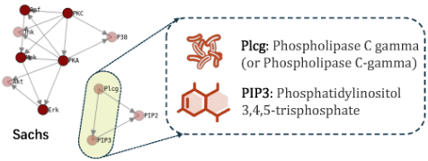
However, is the score function can be applied across various scenarios? To explore this, we still take BIC [Schwarz, 1978] as example and consider the limited sample size case, which frequently arises in medical field. As illustrated in Figure 1 [Sachs et al., 2005], BIC exhibits varying preferences in model selection depending on the sample size. In fact, this gap is universal across score functions used for model selection. For instance, abnormal noise can negatively impact the BIC-Gaussian score, and the choice of priors can influence the BDeu score. Although some improvements have been proposed under various conditions [Silander et al., 2008; Huang et al., 2018; Andrews et al., 2018]. it is impractical to manually design new scoring functions for every emerging scenario. Given these challenges, our aim is to improve the score functions in a automatic and systematic manner. In fact, this task can be also framed as an optimization problem, requiring to explore the landscape of possible scoring functions.
Previously, such optimization tasks have been hindered by the lack of a comprehensive understanding of the score function space. Fortunately, recent advancements in large language model (LLM) [Achiam et al., 2023; Zhao et al., 2023] offer promising tools. LLM encodes algorithms through code implementation and contextual description, enabling more effective search methods for algorithm design [Liu et al., 2024b; Romera-Paredes et al., 2024]. Inspired by it, we propose the L-SFE (LLM-enhanced Score Function Evolution) framework to discovery optimal score functions. Note that L-SFE still achieves the MEC-level identifiability under the causal faithfulness and causal suffiency assumptions [Pearl, 2009]. The contribution of this paper includes:
- We frame L-SFE as a supervised learning process and formulate it using a bi-level optimization approach. At the lower level, a greedy local search (GLS) is employed to identify the optimal DAGs based on the specific score function. At the upper level, Evolutionary algorithm (EA) is utilized to optimize the scoring function with maximal fitness, which is quantified by the structural difference between the aforementioned DAGs and the ground-truth graphs.
- For LLM, we take the BIC as standard and design the prompt integrating both conceptual and code-level information to initialize and evolve the scoring function. Additionally, we refine several operators, including mutation, crossover, and injection, to effectively balance convergence and diversity of EA.
- We evaluate the generated scoring functions from both theoretical and experimental analysis. The former focuses on equivalence and consistency, while latter is performed across synthetic (including discrete and continuous) and real-world data. The results demonstrate the effectiveness, stability, and generality of L-SFE.
2 RelatedWorks
Causal Structure Learning. The score-based CSL algorithms can be categorized into combination-based and continuous-based types. The former execute approximate or exact search in: (1) DAG space G (e.g., HC [Heckerman et al., 1995] and MAHC [Constantinou et al., 2022]), which explore plausible DAGs by heuristically manipulating single or multiple directed edges; (2) EC (Equivalent space) space E (e.g., GES [Chickering, 2002] and fGES [Ramsey et al., 2017]), which greedy search the completely partially directed acyclic graph (CPDAG) via forward equivalent search and backward equivalent search. (3) Permutation space O (e.g., OBS [Teyssier and Koller, 2012], GRaSP [Lam et al., 2022], and BOSS [Andrews et al., 2023]), which identify the best causal structure by discovering the topological ordering that maximizes ancestral information. Continuous-based algorithms make assumptions about the data distribution and learn causal graphs from a structural equation model (SEM), such as LiNGAM [Shimizu et al., 2011], NOTEARS [Zheng et al., 2018], DAG-RL [Zhu et al., 2019] and DAGMA [Bello et al., 2022] et al.
LLM for CSL. Given the exceptional text comprehension capabilities, numerous studies have leveraged LLM to research the causality [Kıcıman et al., 2023; Takayama et al., 2024]. These approaches regard LLM as sole determiners of pairwise causal relationships [Zhiheng et al., 2022; Wan et al., 2024] or domain experts. The latter harness metainformation embedded in the LLM's training data to enhance the causal discovery, including initialization [Ban et al., 2023; Li et al., 2024], post-door adjustments [Khatibi et al., 2024], or structural constraints fusion [Ban et al., 2023; Zhou et al., 2024; Jiralerspong et al., 2024; Zhang et al., 2024].
LLM for Algorithm Design. Finally, we provide a brief overview of using LLM for auto algorithm design. Most existing frameworks employ evolutionary approaches and leverage operators defined within the algorithmic space for algorithm generation, such as FunSearch [Romera-Paredes et al., 2024], EoH [Liu et al., 2024b], and ReEov [Ye et al., 2024]. Additionally, these frameworks have been applied to a variety of scenarios, including the capacitated vehicle routing problem [Liu et al., 2024a], critical node discovery [Mao et al., 2024], and tensor network search [Zeng et al., 2024].
3 Background
DAG can be described as a tuple G = (V ,E), where V = {X1,X2, · · · ,Xn} represents the collection of variables, and E = {Xi → Xj|Xi,Xj ∈ V } denotes the directed edges between the variables. CSL can be typically formulated as the optimization problem
Ψ(.) is a score function that evaluates the fitness of DAG G on i.i.d dataset D = {D1, · · · ,Dm}, and it is usually decomposable and equivalence [Koller, 2009].
Definition 1. (Decomposable) If the score functionΨ(G|D) can be written as Ψ(G|D) = ∑Xi∈V Ψ(Xi, PaGi |D), then Ψ is decomposable.
Definition 2. (Equivalence) ∀G1, G2 ∈ G, if G1, G2 is Iequivalent, and Ψ(G1|D) = Ψ(G2|D) holds, then Ψ is equivalence.
where PaGi represent the parents of Xi in G. For discrete datasets, the most commonly used information theoretic score functions include BIC and AIC [Kitson et al., 2023], which evaluate model based on the multi-information content and entropy of the variables. Other Bayesian scores, such as BDeu, BDs, K2, and BDe[Kitson et al., 2023], place priors on the parameters of the tabular conditional probability distribution. For continuous datasets, BIC remains applicable when using conditional covariance matrix. Thus, we take BIC as benchmark for evolution [Andrews et al., 2023]
where ℓ(.) is a log-likelihood function, and ˆ θmle represents the maximum likelihood estimation (MLE) for the parameters of subgraph Gi : PaGi → Xi. Furthermore, BIC is also consistent if the underlying distribution P behind D belongs to a curved exponential family [Haughton, 1988].
Definition 3. (Consistent) Suppose G ∗ is a P-map under the distribution P ∗ . A score function Ψ is said to be consistent if as the sample size m→∞, the following conditions hold:
- The structure G ∗ maximum the Ψ(G ∗ |D).
- ∀G ∈ G, if G is not I-equivalent to G ∗ , then Ψ(G|D) < Ψ(G ∗ |D).
4 Framework
The search in score function space can be formulated as a bi-level optimization problem
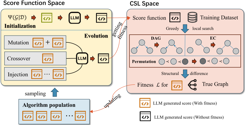
where G ∗ denotes the arbitrary DAG within G, and DG∗ represents the dataset sampled from G ∗ under the gaussian or multinational distribution. Dis(Ga, Gb) is a structural distance measure for Ga, Gb. Note that in equation 3, the upper level optimization identify the optimal Ψ by minimizing the expectation of structural loss over all possible G ∗ assigned with DG∗ . This objective can be achieved through lower level optimization, which finds the best G †Ψ,DG∗ for a given score function Ψ. Furthermore, since the score function space is abstract, L-SFE employes EA to solve equation 3, as it does not require a clear characterization for the mathematical properties of the solution. As shown in figure 2, the workflow of the L-SFE can be divided into two stages. Firstly, EA searches the score function space to identify an improved Ψ; then, Ψ is combined with the GLS to solve the lower level optimization problem, ultimately leading to a best DAG for evaluating the fitness of Ψ.
4.1 Score Function Generation
In this subsection, we provide a detailed explanation of how the score function is discovered using LLM.
Prompts Design. Inspired by EoH [Liu et al., 2024b], all prompts pt are designed using a three-level hierarchical structure as shown in figure 3. Task Description informs the LLM of its intended role and the objective of CSL. Code Snippets presents few-shot examples to heuristic the LLM designing analogous score functions, and it contains two key components: Idea, which provides a textual explanation of the core thought behind the score function; Code, which presents the detailed Python implementation. In addition, there is an optional item that demonstrates the fitness of the score function. Task Assignment applies the chain-of-thought (CoT) reasoning [Wei et al., 2022] to derive better scoring functions from the given examples, and it includes four steps:
- First, the LLM carefully reads and interprets the core idea provided in the code comments;
- Second, if the input score function is labeled with a fitness, the LLM analyzes the reasons behind its effectiveness or shortcomings;
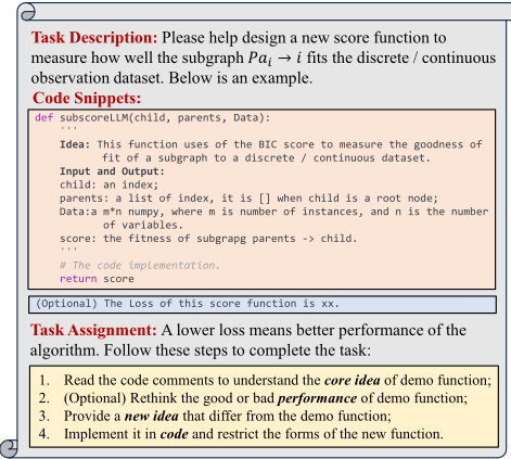
- Third, based on the selected operators, different prompts are generated to inspire new ideas that diverge from the given examples;
- Finally, the LLM implements the new idea in code, ensuring that the function name, input, and output match those in the example code.
Fitness Evaluation inCSLSpace. Based on equation 3, LSFE employs the Monte Carlo method [Metropolis and Ulam, 1949] to randomly sample np ground-truth graphs G ∗ and corresponding training datasets DG∗ for training. For convenience, the weight matrix W k ∈ {0, 1}n×n is used to represent the k-th G ∗ , where W k ij = 1 implies the directed edge Xi → Xj, and the sampled dataset is denoted as Dk . Then, the Normalized Hamming Distance [Kıcıman et al., 2023] is used to quantify the Dis(Ga, Gb). Thus, the fitness function can be formulated as
where dW k denotes the number of variables in W k . W †Ψ,Dk represents the best DAG learned by the pre-selected GLS under Ψ and Dk . Obviously, a lower L(Ψ) indicates a higher fitness. Note that GLS can source from different CSL spaces, such as HC in DAG space, GES in EC space and BOSS in permutation space.
EA in Score Function Space. The initial algorithm population Ψ = {Ψ1, · · · ,Ψna } is generated with standard BIC, and mutation, crossover, and injection are employed for evolution. More detailed prompt design can be referred in Supplementary material 1.1 1 .
1 https://github.com/wzd2502/L-SFE
The crossover operator facilitates the random combination of two score functions, generating a new one that exhibits different structural and conceptual features. Specifically, Ψ1 and Ψ2 are randomly selected from the Ψ. Based on their code implementations and the associated fitness L(Ψ1) and L(Ψ2), LLM analyses and assimilates the ideas of parents to creates a new score function Ψ′ .
The mutation operator modifies an existing score function to generate a variant with potentially altered characteristics. Specifically, Ψ1 is randomly selected from the Ψ with its corresponding fitness L(Ψ1). Based on the extent of the modifications, mutation can be classified into two types: (1) structural mutation, which involves significant alterations to the score function's underlying structure, and (2) parameter mutation, which only modifies the parameters of the score function without altering its fundamental structure.
The injection operator is designed to maintain diversity within the algorithm population, preventing EA convergence to a local optima. Specifically, a new score function Ψ′ is generated, which is entirely distinct from all previous Ψ ∈ Ψ. L(Ψ′ ) is not evaluated at this stage, meaning Ψ′ is directly incorporated into the mutation and crossover operations. Ψ′ will only be discarded at the end of the iteration if it does not contribute positively to the evolutionary.
In each iteration, all of the aforementioned operators are applied repeatedly, and the generated score functions are tested for legality, ensuring that they do not introduce cyclic graphs and can produce results within a specified time limit. After completing an iteration, the population Ψ would be updated. Only the top na algorithms are retained for the next iteration. The evolution continues until a predefined stopping condition is met. To provide a clear understanding of L-SFE, we outline the pseudo-code in Alg. 1 in Supplementary material 1.2.
4.2 Score Function Analysis
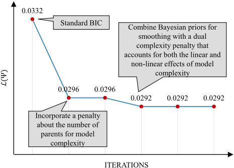
L-SFE is repeated nl times on different training datasets. To avoid ambiguity, we introduce the notation L-SFEabk , a ∈ {D,C}, b ∈ {1, · · · , nl}, k ∈ {1, · · · , na}. This represents the k-th score function learned by L-SFE over the last iteration in b-th repetitions under the a-type dataset (D for Discrete and C for Continuous). Here we take the L-SFED1 as example and analyze its evolution in figure 4, and more detailed results can be found in Supplementary material 1.3.
At the first iteration, L-SFE enhances the CSL by incorporating extra penalty terms that account for the length of the parent sets
Equation 5 modifies only the structure of the penalty, so it remains a consistent and equivalent score. At the end of the evolution, L-SFE identifies an optimal Ψ by incorporating priors into the BIC score, which can effectively mitigate overfitting under limited data. Furthermore, a quadratic penalty is introduced to enhance the model's preference for simplicity, and the penalty term related to the number of data is modified from log(m) to 1/m. This formulation is expressed as
where ˆ θMAP represents the maximum a posterior (MAP) estimate, which is based on Dirichlet prior. Notably, the score function in Equation 6 is decomposable and possesses several advantageous properties
Theorem 1. Score function Equation 6 is still consistent but not equivalence.
The proof can be found in supplementary material 1.3. Actually, all LLM learned scores provide similar insights: they leverage the prior to enhance robustness under limited data and use 1/m rather than log(m) to penalize the graph's complexity in a less restrictive manner.
5 Experiment
5.1 Settings
Datasets. GPT-4o mini is utilized for score function discovery in L-SFE, and synthetic datasets generated from pytetrad are employed for training and testing 2 . For the discrete dataset, L-SFE is trained on ten RandomGraphs with n = 30, where the variables follow a multinomial distribution, and tested on ErdosRenyi (ER) and ScaleFree (SF) graphs. For the continuous datasets, L-SFE is trained on ten RandomGraphs under the linear Gaussian SEM assumption with n = 30, and evaluation is performed on the linear exponential SEM and the linear gumbel SEM. The GLS used for training is HC with a tabu search. Each test is repeated 10 times with m = 5000. Additional details of experimental setup are provided in Supplementary material 2.1.
2 Code is avaliable on https://github.com/wzd2502/L-SFE
Metrics. We evaluate the structural accuracy of L-SFE learned graph against the ground-truth graphs using the Structural Hamming Distance (SHD), the F1 score for adjacency accuracy (F1adj ), and the F1 score for arrow accuracy (F1arr ).
Baselines. The score function generated by L-SFE is compared with commonly used scores, including BIC, BDeu, and BDs for discrete data [Kitson et al., 2023], and BIC-Gaussian for continuous data [Kitson et al., 2023]. Additionally, these methods are integrated with GLS across various search spaces and compared to baseline algorithms, including:
- Discrete. HC [Heckerman et al., 1995], PC [Colombo et al., 2014], BOSS [Andrews et al., 2023], fGES [Ramsey et al., 2017], GRaSP [Lam et al., 2022].
- Continuous. LinGAM [Shimizu et al., 2011], DAGMA [Bello et al., 2022], BOSS, fGES, HC.
5.2 Overall Analysis
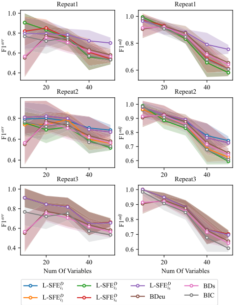
In this subsection, we want to answer the following questions: Stability: Are the all score functions identified by L-SFE consistently superior to human-designed scores? In this topic, we conduct nl = 3 repetitions of L-SFE and record the all na algorithms identified in the last iteration of each repetition. HC is employed as the search method. Figure 5
| ER-10 | ER-20 | ER-30 | ER-40 | ER-50 | SF-10 | SF-20 | SF-30 | SF-40 | SF-50 | |
|---|---|---|---|---|---|---|---|---|---|---|
| PC | 1.1 | 14.4 | / | 112.3 | 200.8 | 8.6 | 34.2 | 50.0 | 136.4 | 163.6 |
| HC | 1.3 | 13.0 | 39.3 | 99.4 | 158.0 | 11.6 | 33.6 | 42.0 | 126.6 | 152.1 |
| BOSS | 1.2 | 6.9 | 31.9 | 87.6 | 149.3 | 10.3 | 35.9 | 44.1 | 130.8 | 156.8 |
| GRaSP | 0.8 | 11.1 | 33.2 | 86.7 | 151.8 | 7.8 | 32.8 | 42.0 | 128.3 | 155.4 |
| fGES | 0.5 | 8.6 | 32.2 | 86.7 | 159.2 | 10.5 | 34.7 | 43.2 | 130.4 | 155.2 |
| L-SFED∗ (G) | 4.7 | 10.8 | 21.4 | 69.1 | 117.5 | 8.0 | 25.9 | 33.8 | 123.3 | 144.8 |
| L-SFED∗∗ (E) | 2.8 | 7.3 | 14.9 | 45.8 | 85.3 | 5.8 | 25.9 | 41.0 | 115.5 | 142.0 |
| L-SFED∗ (O) | 3.4 | 14.1 | 42.9 | 102.7 | / | 5.2 | 21.0 | 48.4 | 130.9 | 156.1 |
| Exp-10 | Exp-20 | Exp-30 | Exp-40 | Exp-50 | Gum-10 | Gum-20 | Gum-30 | Gum-40 | Gum-50 | |
|---|---|---|---|---|---|---|---|---|---|---|
| PC | 14.5 | 23.1 | 35.8 | 39.9 | 37.5 | 12.6 | 18.3 | 27.9 | 37.3 | 50.4 |
| fGES | 12.9 | 28.5 | 38.7 | 33.2 | 17.1 | 13.3 | 17.6 | 21.7 | 27.9 | 28.2 |
| BOSS | 7.1 | 14.6 | 16.1 | 15.8 | 7.8 | 6.2 | 4.5 | 9.3 | 12.1 | 9.2 |
| DAGMA | 17.4 | 40.8 | 56.2 | 61.7 | 76.3 | 22.6 | 39.1 | 54.3 | 65.4 | 79.3 |
| LiNGAM | 3.2 | 6.9 | 9.2 | 13.8 | 17.1 | 4.7 | 11.0 | 21.3 | 24.0 | 32.9 |
| L-SFEC∗ (G) | 14.0 | 22.7 | 59.5 | 31.0 | 23.2 | 14.5 | 19.0 | 32.6 | 46.3 | 38.4 |
| L-SFEC∗ (E) | 12.3 | 29.9 | 37.9 | 34.6 | 20.7 | 12.3 | 15.2 | 19.6 | 21.3 | 27.1 |
| L-SFEC∗ (O) | 9.1 | 3.7 | 7.0 | 8.0 | 8.7 | 0.8 | 2.7 | 5.8 | 8.3 | / |
presents the comparison with three human-designed scores on ER graphs under the discrete dataset, and detailed test results on other settings can be found in Supplementary material 2.2. From figure 5, most of LLM learned score functions are either comparable to or outperform the human-designed scores in each repetition. For instance, L-SFED15 performs best in Repetition 1, while L-SFED21 and L-SFED25 show superior performance in Repetition 2, and L-SFED31 and L-SFED32 lead in Repetition 3. A similar trend is also observed in the SF graphs. In the case of continuous datasets, all score functions learned by the LLM outperform the human-designed BICgaussian score, highlighting the stability of the L-SFE.
Therefore, we select the best score function from i-th repetition, denoted as L-SFEDi∗ and evaluate their generality.
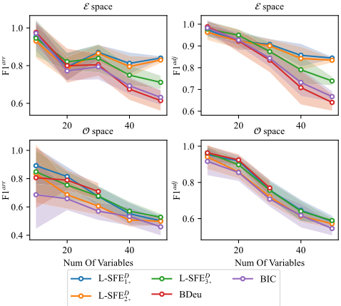
Generality: Can the score functions discovered by L-SFE be applied across different search methods? In this topic, we explore whether the score function, trained using HC in the DAG (G) space, remains effective in the EC (E) and permutation (O) spaces. To investigate this, we employ the GES and BOSS, along with L-SFEDi∗ for testing. The results on ER graphs are displayed in figure 6, with additional results for other settings provided in Supplementary material 2.2. LLM learned score functions still demonstrate strong performance in the EC space as well compared with BIC and BDeu. However, in the permutation space, this superiority narrows significantly. This is likely due to the smaller scope of the permutation space (O(n2n-1 )) compared to the graphical space (O(n!2C2n)), where GLS are more likely to find the optimal solution, with less sensitive to the choice of score function. Notably, the computation cost of the GrowShrink Tree (GST) for BDeu is prohibitively high, preventing BOSS from identifying a DAG in test datasets when n ≥ 40. For the continuous dataset, L-SFE maintains excellent generality in the EC space. However, in the permutation space, due to higher capability of BOSS, L-SFED1∗ and L-SFED2∗ slightly under-perform compared to BIC-gaussian, with only L-SFED3∗ achieving a marginal advantage.
Effectiveness: Does L-SFE improve the performance of CSL compared to state-of-the-art algorithms? Finally, we investigate whether the LLM generated score function, when combined with GLS in different search spaces, can outperform SOTA causal learning methods in tables 1 and 2. Overall, L-SFE achieves the lowest SHD in 8/10 settings on discrete datasets and in 7/10 settings on continuous datasets. Counterexamples are observed in some small-scale networks, such as ER-10, ER-20, and Exp-10. These occurrences are mainly because 5000 instances provide a sufficiently sample size for the BIC to yield optimal results. However, as the problem scale increases, the advantages of L-SFE become more pronounced. For discrete datasets, L-SFE in E space identifies the most optimal DAGs among the eight algorithms, and achieves similar results on continuous datasets in O space. This observation aligns with our understanding that graphical-based GLS are more suited for discrete datasets, whereas permutation-based GLS can explore causal structures in larger steps, making them more effective for SEM causal models. For further results, including F1arr and F1adj scores, please refer to Supplementary material 2.2.
5.3 Other Experiments
Case Study. We present a case study using data from the real world COVID-19 pandemic in the UK 3 . The data set comprises 866 samples that encompass eight categories, including viral tests, infections, hospitalizations, and related factors. The expert-designed benchmark network includes 17 variables, 37 directed edges, and a maximum node degree of 10. The dataset is discretized using k-means and quartiles discretization, as introduced by [Constantinou et al., 2023]. A graphical accuracy analysis is provided in Table 3. Due to the absence of a predefined distribution, the expert-designed benchmark network is not a P-map for dataset. As a result, most existing algorithms fail to produce high F1 score graphs. Even then, the L-SFE-guided GLS approach can consistently identify more correct edges and accurately orient more arrows across different settings.
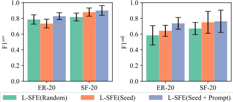
Ablation Study. We investigate howdifferent types of standard score function hints impact the performance of L-SFE under three configurations: 1) Seed + Prompt: The BIC is included in both the population seeds and the code snippets within the prompts; 2) Seed: The initialization code snippets provided only the basic inputs and outputs information, with the BIC placed in the seed; 3) Random Walk: BIC is absent from both the seed and the prompts. Table 3 evaluates their test performance on ER-20 and SF-20. As expected, L-SFE(Prompt + Seed) yields the best F1arr and F1adj , indicating that evolution helps refine the BIC to generate even better score functions, and adding the seed within the population also achieves this goal. However, allowing the LLM to randomly search the score function space leads to suboptimal results. Interestingly, when we extended the number of iterations for L-SFE(RandomWalk) to 10, L-SFE still learn the similar thought of BIC. This observation further supports that BIC represents an optimal solution within the score function space. Furthermore, we also analyze the performance of LSFE across varying sample sizes in Supplementary material 2.2.
3 https://bayesian-ai.eecs.qmul.ac.uk/bayesys/
| k-means | quartiles | |||
|---|---|---|---|---|
| F1arr | F1adj | F1arr | F1adj | |
| PC | 0.235 | 0.441 | / | / |
| HC | 0.419 | 0.581 | 0.194 | 0.451 |
| BOSS | 0.172 | 0.483 | 0.201 | 0.448 |
| GRaSP | 0.142 | 0.500 | 0.250 | 0.463 |
| fGES | 0.264 | 0.415 | ∗ 0.302 | 0.453 |
| L-SFED∗ (G) | 0.253 | 0.507 | 0.347 | 0.533 |
| L-SFED∗ (E) | 0.257 | ∗ 0.571 | 0.225 | ∗ 0.507 |
| L-SFED∗ (O) | ∗ 0.338 | 0.479 | 0.250 | 0.417 |
6 Conclusion
In this paper, we introduce the L-SFE, which leverages LLM and EA to explore the score function space through a bi-level optimization framework. Three key insights from this work are concluded as follows:
- LLM can effectively learn valuable components, such as Dirichlet priors and relaxed penalties. These components are theoretically well-founded and align with human-like reasoning.
- EA are crucial for finding optimal solutions. Even in the absence of explicit guidance, LLM can discover similar principles through iterative refinement.
- The score function space is highly abstract and potentially multimodal, making best-of-n search a valuable approach for yielding improved results.
Although L-SFE focuses primarily on exploring the structure of score functions, additional work is required to optimize their parameters using LLM. Furthermore, future research could focus on guiding LLM in exploring more efficient causal search strategies or expanding the search space beyond conventional frameworks.
@inproceedings{ijcai2025p1010,
  title     = {LLM-enhanced Score Function Evolution for Causal Structure Learning},
  author    = {Wang, Zidong and Liu, Fei and Feng, Qi and Zhang, Qingfu and Gao, Xiaoguang},
  booktitle = {Proceedings of the Thirty-Fourth International Joint Conference on
               Artificial Intelligence, {IJCAI-25}},
  publisher = {International Joint Conferences on Artificial Intelligence Organization},
  editor    = {James Kwok},
  pages     = {9086--9094},
  year      = {2025},
  month     = {8},
  note      = {Main Track},
  doi       = {10.24963/ijcai.2025/1010},
  url       = {https://doi.org/10.24963/ijcai.2025/1010},
}
TY - CPAPER TI - LLM-enhanced Score Function Evolution for Causal Structure Learning AU - Wang, Zidong AU - Liu, Fei AU - Feng, Qi AU - Zhang, Qingfu AU - Gao, Xiaoguang T2 - Proceedings of the Thirty-Fourth International Joint Conference on Artificial Intelligence, IJCAI-25 PB - International Joint Conferences on Artificial Intelligence Organization PY - 2025 SP - 9086 EP - 9094 DO - 10.24963/ijcai.2025/1010 UR - https://doi.org/10.24963/ijcai.2025/1010 ER -Copied
Machine-readable versions of this paper, for tools and AI agents:





