
Efficient Constraint-based Window Causal Graph Discovery in Time Series with Multiple Time Lags
Proceedings of the Thirty-Fourth International Joint Conference on Artificial Intelligence. Main Track. Pages 9095-9103.
https://doi.org/10.24963/ijcai.2025/1011
Keywords
- Machine Learning: ML: Causality
- Knowledge Representation and Reasoning: KRR: Causality
- Uncertainty in AI: UAI: Causality, structural causal models and causal inference
Abstract
We address the identification of direct causes in time series with multiple time lags, and propose a constraint-based window causal graph discovery method. A key advantage of our method is that the number of required conditional independence (CI) tests scales quadratically with the number of sub-series. The method first uses CI tests to find the minimum trek lag between two arbitrary sub-series, followed by designing an efficient CI testing strategy to identify the direct causes between them. We show that the method is both sound and complete under some graph constraints. We compare the proposed method with typical baselines on various datasets. Experimental results show that our method outperforms all the counterparts in both accuracy and running speed.
- [Assaad et al., 2022] Charles K Assaad, Emilie Devijver, and Eric Gaussier. Survey and evaluation of causal discovery methods for time series. Journal of Artificial Intelligence Research, 73:767-819, 2022.
- [Ay and Polani, 2008] Nihat Ay and Daniel Polani. Informa- tion flows in causal networks. Advances in complex systems, 11(01):17-41, 2008.
- [Cai et al., 2024] Ruichu Cai, Yunjin Wu, Xiaokai Huang, Wei Chen, Tom ZJ Fu, and Zhifeng Hao. Granger causal representation learning for groups of time series. Science China Information Sciences, 67(5):152103, 2024.
- [Chen et al., 2024] Mingjie Chen, Hongcheng Wang, Ruxin Wang, Yuzhong Peng, and Hao Zhang. Cdrm: Causal disentangled representation learning for missing data. Knowledge-Based Systems, 299:112079, 2024.
- [Entner and Hoyer, 2010] Doris Entner and Patrik O. Hoyer. On causal discovery from time series data using fci. 2010.
- [Gong et al., 2022] Wenbo Gong, Joel Jennings, Cheng Zhang, and Nick Pawlowski. Rhino: Deep causal tem- poral relationship learning with history-dependent noise. arXiv preprint arXiv:2210.14706, 2022.
- [Gong et al., 2023] Chang Gong, Di Yao, Chuzhe Zhang, Wenbin Li, and Jingping Bi. Causal discovery from tem- poral data: An overview and new perspectives. ArXiv, abs/2303.10112, 2023.
- [Granger, 1969] Clive WJ Granger. Investigating causal rela- tions by econometric models and cross-spectral methods. Econometrica: journal of the Econometric Society, pages 424-438, 1969.
- [Granger, 1980] C.W.J. Granger. Testing for causality: A personal viewpoint. Journal of Economic Dynamics and Control, 2:329-352, 1980.
- [Huang and Kleinberg, 2015] Yuxiao Huang and Samantha Kleinberg. Fast and accurate causal inference from time series data. In Proceedings of the Twenty-Eighth Inter- national Florida Artificial Intelligence Research Society Conference, FLAIRS 2015, Hollywood, Florida, USA, May 18-20, 2015, pages 49-54. AAAI Press, 2015.
- [Hyvärinen et al., 2010] Aapo Hyvärinen, Kun Zhang, Shohei Shimizu, and Patrik O. Hoyer. Estimation of a struc- tural vector autoregression model using non-gaussianity. J. Mach. Learn. Res., 11:1709-1731, aug 2010.
- [Kevin B. Korb and Ann E. Nicholson. Bayesian artificial intelligence, second edition. 2010. Lanne et al., 2017] Markku Lanne, Mika Meitz, and Pentti Saikkonen. Identification and estimation of non-gaussian structural vector autoregressions. Journal of Econometrics, 196(2):288-304, 2017.
- [Malinsky and Spirtes, 2018] Daniel Malinsky and Peter Spirtes. Causal structure learning from multivariate time se- ries in settings with unmeasured confounding. In Proceed- ings of 2018 ACM SIGKDD workshop on causal discovery, pages 23-47. PMLR, 2018.
- [Mastakouri et al., 2021] Atalanti A Mastakouri, Bernhard Schölkopf, and Dominik Janzing. Necessary and sufficient conditions for causal feature selection in time series with latent common causes. In International Conference on Machine Learning, pages 7502-7511. PMLR, 2021.
- [Nauta et al., 2019] Meike Nauta, Doina Bucur, and Christin Seifert. Causal discovery with attention-based convolu- tional neural networks. Machine Learning and Knowledge Extraction, 1(1):312-340, 2019.
- [Pamfil et al., 2020] Roxana Pamfil, Nisara Sriwattana- worachai, Shaan Desai, Philip Pilgerstorfer, Konstantinos Georgatzis, Paul Beaumont, and Bryon Aragam. Dynotears: Structure learning from time-series data. In AISTATS, vol- ume 108 of Proceedings of Machine Learning Research, pages 1595-1605. PMLR, 26-28 Aug 2020.
- [Pearl, 2009] Judea Pearl. Causality. Cambridge University Press, 2 edition, 2009.
- [Peters et al., 2017] Jonas Peters, Dominik Janzing, and Bern- hard Schlkopf. Elements of Causal Inference: Foundations and Learning Algorithms. The MIT Press, 2017.
- [Pfister et al., 2019] Niklas Pfister, Peter Bühlmann, and Jonas Peters. Invariant causal prediction for sequential data. Journal of the American Statistical Association, 114(527):1264-1276, 2019.
- [Prill et al., 2010] Robert J Prill, Daniel Marbach, Julio Saez- Rodriguez, Peter K Sorger, Leonidas G Alexopoulos, Xi- aowei Xue, Neil D Clarke, Gregoire Altan-Bonnet, and Gustavo Stolovitzky. Towards a rigorous assessment of systems biology models: the dream3 challenges. PloS one, 5(2):e9202, 2010.
- [Ramsey, 2014] Joseph D Ramsey. A scalable conditional independence test for nonlinear, non-gaussian data. arXiv preprint arXiv:1401.5031, 2014.
- [Runge et al., 2019] Jakob Runge, Peer Nowack, Marlene Kretschmer, Seth Flaxman, and Dino Sejdinovic. Detecting and quantifying causal associations in large nonlinear time series datasets. Science advances, 5(11):eaau4996, 2019.
- [Runge, 2018] Jakob Runge. Causal network reconstruction from time series: From theoretical assumptions to prac- tical estimation. Chaos: An Interdisciplinary Journal of Nonlinear Science, 28(7):075310, 2018.
- [Runge, 2020] Jakob Runge. Discovering contemporaneous and lagged causal relations in autocorrelated nonlinear time series datasets. In Conference on Uncertainty in Artificial Intelligence, pages 1388-1397. PMLR, 2020.
- [Sachs et al., 2005] Karen Sachs, Omar Perez, Dana Pe'er, Douglas A Lauffenburger, and Garry P Nolan. Causal protein-signaling networks derived from multiparameter single-cell data. Science, 308(5721):523-529, 2005.
- [Shimizu et al., 2006] Shohei Shimizu, Patrik O Hoyer, Aapo Hyvärinen, and Antti Kerminen. A linear non-gaussian acyclic model for causal discovery. The Journal of Machine Learning Research, 7:2003-2030, 2006.
- [Spiegelhalter et al., 1993] David J. Spiegelhalter, A. Philip Dawid, Steffen L. Lauritzen, and Robert G. Cowell. Bayesian Analysis in Expert Systems. Statistical Science, 8(3):219 -247, 1993.
- [Spirtes et al., 2000] Peter Spirtes, Clark N Glymour, and Richard Scheines. Causation, prediction, and search, vol- ume 81. MIT press, 2000.
- [Sugihara et al., 2012] George Sugihara, Robert May, Hao Ye, Chih hao Hsieh, Ethan Deyle, Michael Fogarty, and Stephan Munch. Detecting causality in complex ecosys- tems. Science, 338(6106):496-500, 2012.
- [Sullivant et al., 2010] Seth Sullivant, Kelli Talaska, and Jan Draisma. Trek separation for gaussian graphical models. The Annals of Statistics, pages 1665-1685, 2010.
- [Sun et al., 2023] Xiangyu Sun, Oliver Schulte, Guiliang Liu, and Pascal Poupart. Nts-notears: Learning nonparametric dbns with prior knowledge. Proceedings of The 26th Inter- national Conference on Artificial Intelligence and Statistics, pages 1942-1964, 2023.
- [Xu et al., 2024] Wenwei Xu, Hao Zhang, Yewei Xia, Yixin Ren, Jihong Guan, and Shuigeng Zhou. Hybrid causal feature selection for cancer biomarker identification from rna-seq data. IEEE/ACM Transactions on Computational Biology and Bioinformatics, 2024.
- [Zhang et al., 2012] Kun Zhang, Jonas Peters, Dominik Janz- ing, and Bernhard Schölkopf. Kernel-based conditional in- dependence test and application in causal discovery. arXiv preprint arXiv:1202.3775, 2012.
- [Zhang et al., 2017] Hao Zhang, Shuigeng Zhou, Kun Zhang, and Jihong Guan. Causal discovery using regression-based conditional independence tests. In AAAI, pages 1250-1256, 2017.
- [Zhang et al., 2021] Hao Zhang, Kun Zhang, Shuigeng Zhou, Jihong Guan, and Ji Zhang. Testing independence between linear combinations for causal discovery. In Proceedings of the AAAI conference on artificial intelligence, volume 35, pages 6538-6546, 2021.
- [Zhang et al., 2024] Hao Zhang, Yixin Ren, Yewei Xia, Shuigeng Zhou, and Jihong Guan. Towards effective causal partitioning by edge cutting of adjoint graph. IEEE Transactions on Pattern Analysis and Machine Intelligence, 46(12):10259-10271, 2024.
- [Zheng et al., 2018] Xun Zheng, Bryon Aragam, Pradeep Ravikumar, and Eric P. Xing. Dags with NO TEARS: con- tinuous optimization for structure learning. In Advances in Neural Information Processing Systems, pages 9492-9503, 2018.
References were extracted automatically from the PDF and may contain errors.
Full text extracted automatically from the PDF; figures, tables and equations may differ. The PDF is the version of record.
1 Introduction
Causal discovery from time series is a fundamental problem in many fields of science and engineering, e.g. economics, bioinformatics, and climate research [Xu et al., 2024; Chen et al., 2024]. In contrast to the stationary cases [Zhang et al., 2024], causal discovery from time series is partially less and partially more challenging [Runge et al., 2019]. In practice, temporal order significantly facilitates the identification of causal directions for lagged links. Meantime, it also faces significant challenges, including high-dimensionality, nonlinear dependencies, multiple lagged dependencies, and so on [Mastakouri et al., 2021]. Several approaches are addressing the problem of time-series causal discovery, including summary causal graph and window causal graph discovery [Assaad et al., 2022], among which Granger causality-based [Granger, 1969; Cai et al., 2024], noise-based methods [Hyv¨arinen et al., 2010], score-based methods [Pamfil et al., 2020] and constraint-based [Runge, 2020] or conditional independence
(CI) based methods [Zhang et al., 2017] form the main pillar. Although these methods have achieved some success in certain scenarios under different assumptions, they still face several problems. Granger causality-based methods have misleading issues in some scenarios [Peters et al., 2017; Ay and Polani, 2008]. Score-based and noise-based methods typically exploit some assumptions of the causal mechanisms or noise distributions. However, in real-world data, the assumed causal mechanisms and distribution forms may not hold, which largely restricts their applications [Zhang et al., 2021]. Besides, previous constraint-based methods such as PCMCI [Runge et al., 2019] have a high time complexity. Last but not least, almost all these methods (except for PCMCI) assume only one single time lag exists explicitly or implicitly, which rarely occurs in complex dynamic systems.
In this work, we focus on the constraint-based technique to discover window causal graphs in time series data with multiple time lags, without assuming particular causal mechanisms or data distributions. To boost efficiency, we develop a pruning strategy by reducing the number of CI tests based on fast-revealed minimum trek lag (see definition in Sec. 3).
Our main theoretical contributions include 1) providing the necessary and sufficient conditions for identifying causal relationships from time series with multiple time lags, and 2) proving that the subsequently proposed algorithm has a time complexity of O(d 2 TCI) where d is the number of subseries, TCI is the time complexity of the chosen CI test algorithm. Our practical contributions lie in 1) extensive numerical experiments with performance comparison with typical Granger causality-based, noise-based, score-based, and constraint-based methods, and 2) the open-source implementation of our time series causal discovery algorithm.
2 Preliminaries
We consider a d-variate discrete-time stochastic process Xt∈T where T stands for the index set. For a fixed time point t ∈ T, Xt = (X 1 t , ..., X d t ), X p t represents a measurement of the p-th time sub-series at time t. We use X p to refer to the p-th time sub-series when there is no need to specify its time t. In what follows, we review some terminologies of the associations between time series and causal modeling. Causality concepts used here without explicit definition, such as causal graphs, which can refer to standard literature [Pearl, 2009].
Definition 1. (Full-time causal graph). Let Xt∈T be a dvariate discrete-time stochastic process and Gfull = (V, E) the associated full-time causal graph. The set of vertices V consists of the set of components X 1 , ..., X d at each time t ∈ T. There is an edge X p t → X q t+ ν ∈ E if and only if X p t causes X q t+ ν , i.e. X p t ∈ PA(X q t+ ).
ν
For a full-time causal graph, we usually set index set T to Z. Then it is generally impossible to infer full-time causal graphs as there usually exists a single observation for each time series at each time instant [Malinsky and Spirtes, 2018]. To remedy this, in time-series causal discovery, it is common to rely on causal stationarity assumption [Runge, 2018].
Definition 2. (Causal stationarity). A multivariate discretetime stochastic process Xt∈T is said to satisfy the causal stationarity assumption if X follows a stationary discrete-time structural vector-autoregressive process that remains invariant throughout the time, which is described by the following structural causal model (SCM):
where f denotes any real-valued multivariate function, and ϵ p t represents the noise variable independent from all X p t 's causal parents PA(X p t ).
In this paper, we assume ∀p ∈ [1, d], t ∈ T, ϵ p t are mutually independent. Under the causal stationarity assumption, the full-time causal graph can be simplified to a finite graph, commonly referred to as the window causal graph. In what follows, if not specified for the full-time graph, we assume the index set T is a finite set with size T.
Definition 3. (Window causal graph) [Assaad et al., 2022]. Let Xt∈[1,T] be a d-variate discrete-time stochastic process and Gw = (V, E) the associated window causal graph with a window size w. V consists of the set of components X 1 , ..., X d at each time t, · · · , t + w, X p t → X q t+ ν ∈ E if and only if X p t cause X q t+ ν (0 ≤ ν ≤ w).
In some scenarios, it is sufficient to know the causal relations between time series as a whole, without knowing precisely the relations between time instants. In that case, one can further simplify the window causal graph into a summary causal graph.
Definition 4. (Summary causal graph) [Gong et al., 2023]. Let Xt∈[1,T] be a d-variate discrete-time stochastic process and Gs = (V, E) the associated summary causal graph. The set of vertices V consists of the set of components X 1 , ..., X d . There is an edge X p → X q ∈ E if and only if X p causes X q at some time t, i.e., X p t ∈ PA(X q t ′ ) for some t and t ′ (t ≤ t ′ ).
The methods for discovering summary causal graphs are usually interested in only the causal relations between time series without specifying time lags, while the methods for discovering window causal graphs focus on the causal relations between time series with time instants.
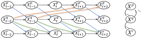
The challenge of multiple time lags. Multiple time lags will cause PA(X p t ) ∩ PA(X p t ′ ) � ∅ for some p with all t � t ′ , making the full-time and window causal graphs more complex and dense. Consequently, multiple time lags not only increase the difficulty of causal discovery, but also highly increase time consumption, especially for constraint-based methods [Runge et al., 2019], which will also be verified by our experiments (Section 5). Some methods like SyPI [Mastakouri et al., 2021] ignore the multiple time lags and only detect the first/minimum one to improve their performance. In this work, our goal is to detect all time lags between different sub-series effectively and efficiently.
3 RelatedWorks
There are four main categories of methods for learning causal graphs in time series data including Granger causality-based, constraint-based, score-based and noise-based methods.
Granger causality [Granger, 1969; Granger, 1980] has been the standard approach in causal analysis of time series for half a century. We can detect that a time series X p Granger-causes X q if the past values of X p provide unique, statistically significant information about future values of X q . Generally, Granger causality cannot deal with contemporaneous links [Peters et al., 2017], and may be problematic in dynamic systems with weakness to moderate coupling, because separability (causes information is not contained in effects) is not always met [Granger, 1969; Sugihara et al., 2012].
Constraint-based methods are largely based on the graphical criterion of d-separation [Spirtes et al., 2000] and CI tests under the causal Markov and faithfulness assumptions. tsFCI [Entner and Hoyer, 2010] and SVAR-FCI [Malinsky and Spirtes, 2018] are both inspired by the FCI algorithm [Spirtes et al., 2000]. tsFCI uses time order and stationarity to restrict conditioning sets and to apply additional edge orientations; SVAR-FCI utilizes stationarity to infer additional edge removals. These methods are computationally intensive due to exhaustive searching over all time lags and conditioning sets, i.e., requiring extensive CI tests [Mastakouri et al., 2021]. PCMCI [Runge et al., 2019] is a more efficient constraintbased method, which first constructs a partially connected graph, then removes all unnecessary edges by testing CIs, finally deals with the autocorrelations by using the Momentary Conditional Independence (MCI) test.
Score-based methods are developed based on Structural Equation Models (SEM), describing a causal system by a set of equations, each of which explains one variable of the system in terms of its direct causes and some additional noise.
Among the existing score-based methods, the recent continuous optimization-based methods DYNOTEARS [Pamfil et al., 2020] and NTS-NOTEARS [Sun et al., 2023] should stand for the state-of-the-art. They revolve around minimizing a penalized loss subject to an acyclicity constraint by leveraging a recent algebraic result characterizing the acyclicity constraint as a smooth equality constraint [Zheng et al., 2018].
For noise-based methods, [Hyv¨arinen et al., 2010] introduced a temporal extension of LiNGAM [Shimizu et al., 2006], called VarLiNGAM. [Huang and Kleinberg, 2015] extended VarLiNGAM by considering linear and nonlinear time-varying models. Recently, [Lanne et al., 2017] generalized the initial VarLiNGAM by considering graphs that may contain cycles.
Some causal feature selection methods focus on the causal relations regarding the target series, which sometimes can be treated as a subtask of causal discovery. The most well-known methods are seqICP [Pfister et al., 2019] and SyPI [Mastakouri et al., 2021]. seqICP requires sufficient interventions in the dataset while SyPI removes this limitation and works efficiently in the case of a single time lag with latent confounders.
4 Method
For a multivariate discrete-time stochastic process X, our goal is to discover the underlying window causal graph Gw = (V, E) by detecting the parents of each X p t (t ∈ T), i.e. the PA(X p t ) in Eq. (1). In what follows, we first introduce some terminologies and notations.
Terminology notation:
- T1. X p t → X q t ′ (t ≤ t ′ ∈ T) means a directed edge in the full-time graph (Def.1), i.e., X p t directly causes X p t ′ .
- T2. X p t � X q t ′ (t ≤ t ′ ∈ T) means a directed path that may contain intermediate nodes in the full-time graph, i.e., X p t is either a direct or indirect cause of X p t ′ .
- T3. X p t - - - X q t+ ν (t, t + ν ∈ T) means a trek, a collider-free path (not necessarily directed) in the full-time graph, i.e., X p t is an ancestor of X q t+ ν , or X p t is one of the descendants of X q t+ , or they share a common ancestor.
ν
- T4. v is a trek lag for the ordered pair (X p , X q ) if there exists a trek X p t - - - X q t+ ν (t, t + ν ∈ T, ν ≥ 0) that does not contain a link of the form X r t ′ → X r t ′ +1 , with arbitrary t ′ , t ′ + 1 ∈ T , r � p, q, nor any duplicate node, and any node in this path does not belong to X p and X q .
- T5. ν is a causal lag for the ordered pair (X p , X q ) if there exists a directed path X p t � X q t+ ν (t, t + ν ∈ T, ν ≥ 0) that does not contain a link of the form X r t ′ → X r t ′ +1 , with arbitrary t ′ , t ′ + 1 ∈ T , r � p, q, nor any duplicate node, and any node in this path does not belong to X p and X q .
- T6. ν is a direct causal lag for the ordered pair (X p , X q ) if there exists a directed edge X p t → X q t+ ν (t, t+ ν ∈ T , ν ≥ 0). For simplicity, we also call ν a time lag throughout the whole paper when no ambiguity exists.
- T7. We say that ν is a non-causal lag for the ordered pair (X p , X q ) if ν is a trek lag but not a causal lag for this pair.
- T8. The maximum time lag τ = max{τpq|∀p � q ∈ [1, d]}, where τpq denotes the maximum time lag for (X p , X q ).
Fig. 1 shows examples of trek lags in time series based on T1-T8. There is a causal lag ν = 2 for (X p , X r ) regarding the path X p t-1 → X q t → X r t+1 , and the path X p t-1 → X q t → X r t+2 defines another causal lag ν = 3 for (X p , X r ). An example for the non-causal lag is ν = 1 for (X r , X p ) regarding the path X p t+2 ← X q t-1 → X r t+1 . Notably, X r t+1 is not a cause of X p t+2 but they still define a trek lag for (X r , X p ). Besides, there are multiple trek lags for (X q , X r ), which are ν = 1 and ν = 2, respectively, shown by X q t → X r t+1 and X q t → X r t+2 . The path X p t-1 → X q t → X q t+1 → X r t+2 does not meet the definition of a trek lag, because it contains a link X q t → X q t+1 .
In this work, T4∼T7 are slightly different from those in some previous works [Mastakouri et al., 2021]. Besides, we use another name "trek lag" instead of "lag" in their paper as in most other papers (e.g., [Gong et al., 2022; Runge et al., 2019]) "lag" means "direct causal lag" (defined in T6) by default. Inspired by [Sullivant et al., 2010] that uses "trek" to represent a collider-free path between two variables, we rename the term to avoid ambiguity. In what follows, we list the assumptions used in this work.
General assumptions:
- A1. Causal Markov condition in the full-time causal graph.
- A2. Causal Faithfulness in the full-time causal graph.
- A3. No backward arrows in time X p t ↛ X q t-ν , ∀ν > 0.
- A4. Acyclic is satisfied in the full-time causal graph.
- A5. Causal stationarity (Def. 2) is satisfied in the full-time causal graph.
- A6. The maximum time lag τ exists in the observed data.
- A7. There is no arrow X p t-ν → X p t for ν > 1.
- A8. No contemporaneous link is contained in the full-time causal graph.
Notice that A1∼A7 are standard assumptions for causal discovery in time series, A8 is an assumption used in many previous works [Mastakouri et al., 2021; Entner and Hoyer, 2010] that cannot detect contemporaneous causal relations. A4 is for the full-time causal graph, acyclic is not necessarily assumed for the summary causal graph (Def. 4). As for A6, if τ is so large that it exceeds T, we naturally cannot test all possible time lags using our observed data. Thus, the methods that can deal with multiple time lags [Runge et al., 2019] usually need to make an additional assumption on τ in the whole X, so does our method. Besides, τ itself can be treated as a hyper-parameter influences performance in the experiments.
In what follows, we introduce the details of the proposed method. Our proposed method consists of two phases: the first phase aims to detect the minimum trek lag (causal or noncausal lag) for every two sub-series, and in the second phase the causal relations are discovered based on these minimum trek lags. We have the following results.
Lemma 1. Given a d-variate discrete-time stochastic process Xt∈[1,T], assuming A1∼ A8 and the maximum time lag τ between two arbitrary sub-series. The minimum non-zero trek lag ν for (X p , X q ) coincides with the minimum non-zero integer ν ′ (1 ≤ ν ′ ≤ τ) that satisfies
except for the following conditions are all satisfied: 1) there is no path defining a trek lag ν ′ for X p t-ν ′ to X q t , and 2) X p has memory, i.e., ∀t, X p t-1 → X p t , and 3) there is a trek between X p t ′ and X q t that does not contain any duplicate node, nor any node in this path belonging to X p and X q .
The proof is provided in the Appendix. Take Fig. 1 as an example, we can find a minimum trek lag v = 2 for (X p , X r ) and also a minimum trek lag v = 1 for (X r , X p ). Lemma 1 summarizes the cases that would fail to detect the true minimum trek lag between two series by testing CI defined in Eq. (2). Besides, Lemma 1 indicates that the minimum trek lag for an arbitrary ordered pair (X p , X q ) can generally be identified by testing at most τ times of the CI test in Eq. (2). If CI tests unfortunately return a false minimum trek lag smaller than the actual minimum trek lag wpq, it will just increase the size of controlling set of some CI tests in the phase of causal discovery. Assuming there are no minimum trek lag returns, we can deduce that no causal link exists from X p to X q given the maximum time lag τ condition.
Next, we investigate the causal relations from X p to X q based on the returned minimum trek lags.
Lemma 2. Given a d-variate discrete-time stochastic process Xt∈[1,T], assuming A1∼ A8 and the maximum time lag τ between two arbitrary variables. Let wpq be the minimum trek lag for (X p , X q ), then X p directly causes X q with a time lag v (v ≥ wpq) if and only if
where Z p = (X p t-v-1 , ..., X p t-wpq ) \ X p t-v , Z q = X q t-1 and ∀r ∈ [1, d] \ {p, q}, Z r = (X r t-τ-1 , ..., X r t-wrq ) where wrq denotes the minimum trek lag for (X r , X q ).
Proof. The necessity is evident by the fact that X p t-v directly causes X q t will lead to X p t-v ̸ � X q t controlling on any other variables. Then, we focus on how to prove the sufficiency by contradiction. First, assume that X p t-v ̸ � X q t |(X q t-1 , Z 1 , ..., Z d ) and X p t-v ↛ X q t , then there are three cases of relations between X p t-v and X q t : 1) there exists an indirect causal link X p t-v � X q t , 2) X p t-v and X q t share a common ancestor, i.e., X p t-v � X r t ′ � X q t , 3) X p t-v and X q t have a collider, i.e., X p t-v � X r t ′ � X q t .
Case 1. (i) If path X p t-v � X q t does not contain any intermediate node (except X p t-v and X q t ) belonging to X p ∪ X q , then Z r containing the direct causes of X q t will block this link, then X p t-v � X q t |(Z 1 , ..., Z d ). (ii) If path X p t-v � X q t contains an intermediate node X q t ′ (t ′ < t) and each node in X q t ′ � X q t belongs to X q , then Z q = X q t-1 will block this link; else if X q t ′ � X q t contains a node from a third series, then Z r containing the direct causes of X q t will also block this link. (iii) If X p t-v � X q t contains X p t ′ where t -wrq < t ′ , then the CI between X p t ′ and X q t is ensured by X p t-v � X q t |(X p 1:(t-v ′ i -1) , X q t-1 ) according to Lemma 1; if t - wrq ≥ t ′ and each node in X p t-v � X p t ′ belongs to X p , then X p t-v+1 ∈ Z p blocks this link, else if X p t-v � X p t ′ contains a node from a third series, then (X p t-v+1 , ..., X p t-w ) ⊂ Z p ) will also block this link.
Case 2. Similarly, we can deduce that X p t-v and X q t are dseparable when X p t-v � X r t ′ � X q t does not contain any intermediate node (except X p t-v and X q t ) belonging to X p ∪ X q , and X p t-v � X r t ′ � X q t contains X q t ′ (t ′ < t). The only case necessitates consideration is when X p t-v � X r t ′ � X q t contains X q t ′ (t ′ < t - v). (i) If each node in X p t ′ � X p t-v belongs to X p , then Z p blocks this link. (ii) If X p t ′ � X p t-v contains a node from a third series X r , when X p t ′ � X p t-v has the form of X p t ′ � X r � X p t-v-1 → X p t-v , then X p t-v-1 ∈ Z p blocks this link; when X p t ′ � X p t-v has the form of X p t ′ � X r t-v-1 → X p t-v , then X r t-v-1 ∈ Z r also blocks this link.
Case 3. Under assumption A3, X p t-v � X r t ′ � X q t exists only when t ′ > t > t - v. Consequently, neither X r t ′ nor its descendent(s) can be contained in (Z 1 , ..., Z d ), thus X p t-v and X q t are d-separable.
Therefore, there is a contradiction in the three cases.
□
Lemma 2 provides the sufficient and necessary conditions Eq. (2) for detecting a direct causal relationship between two sub-series X p and X q given the minimum trek lag wpq for (X p , X q ). For the case of multiple time lags, we just need to test at most τ times of CI test of Eq. (3) by searching v from wpq, wpq + 1, ... to τ, where τ denotes the maximum time lag. Back to Lemma 1, if the CI test of detecting the minimum trek lag unfortunately returns a false one, it will increase the size of controlling set of some CI tests in Eq. (2), leading to more time consumption and lower accuracy. However, this does not affect the soundness and completeness of our method in theory. The final task is to detect the self-connections, as we do not make any assumptions regarding the presence of selfconnections for each time series. This goal can be achieved by the following lemma.
Lemma 3. Given a d-variate discrete-time stochastic process Xt∈[1,T], assuming A1∼ A8, then there is a self causal link X p t-1 → X p t if and only if
where PA(X p t ) is the parent set of X p t .
The proof of Lemma 3 is straightforward, because PA(X q t ) blocks all the connections between X p t-1 and X p t if there is no self-connection.
5 Algorithm
Now, put all the theoretical results above together, we propose a novel method for fast causal discovery in time series with multiple time lags, which is called CDiT (an abbreviation of Causal Discovery in Time series). The process of CDiT is outlined in Alg. 1. Alg. 1 consists of two phases: the first phase aims to detect the minimum trek lag (causal or noncausal lag) for every two sub-series by testing the CI defined in Eq. (2) (Lines 1∼7), and the second phase aims to discover the causal relations based on these minimum trek lags by testing the CI defined in Eq. (3) (Lines 8∼11), and check the selfconnections by testing the CI defined in Eq. (4) (Lines 12∼14). It can be seen that there is only one hyper-parameter τ in Alg. 1 (except the possible hyper-parameters used in the chosen CI
Algorithm 1 CDiT (Causal Discovery in Time series)
Input: A d-variate discrete-time stochastic process Xt∈[1,T]; maximum time lag τ.
- Output: The window graph Gw of X. 1: for ∀X p , X q ∈ X do 2: for wpq = 1 to τ do 3: if X p t-wpq ̸ � X q t |(X p t-wpq-τ , ..., X p t-wpq-1 , X q t-1 ) defined in Eq. (2) holds then 4: save wpq as the minimum trek lag for X p to X q . 5: break 6: else 7: save wpq = ∅. 8: for ∀X p , X q ∈ X and wpq � ∅ do 9: for vpq = wpq to τ do 10: if X p t-vpq ̸ � X q t |(X q t-1 , Z 1 , ..., Z d ) defined in Eq. (3) holds then 11: save vpq as one time lag for X p directly causing X q . 12: for ∀X p ∈ X do 13: if X p t-1 ̸ � X p t |PA(X p t ) \ X p t-1 defined in Eq. (4) holds then 14: save 1 as the time lag for X p directly causing itself. 15: Constructs Gw based on all vpq of ∀X p , X q ∈ X.
test method), which is also a standard parameter required by many previous approaches that can deal with multiple time lags [Runge et al., 2019].
A significant advantage of the proposed method is its high efficiency, we have the following theoretical result:
Lemma 4. The time complexity of Alg. 1 is O(d 2 TCI) where d is the number of sub-series, TCI is the time complexity of the chosen CI test algorithm.
Theoretically, we have to use at least one CI test to check CI between two series, then the total number of CI tests should be at least d(d - 1), leading to O(d 2 TCI) time complexity. So, we have reason to conjecture that Alg. 1 meets the lower bound of the complexity of constraint-based methods. In contrast, PCMCI [Runge et al., 2019] requires O(d 3 TCI) time complexity, which will take significantly longer time than CDiT when d is large.
Discussion. The performance of Alg. 1 highly depends on two high-order CI tests (Lines 3&13 in Alg. 1), which easily cause Type-II error [Ramsey, 2014], i.e. the CI hypothesis is accepted even though it is actually false. We cannot completely avoid this problem but alleviate it by detecting the minimum trek lags (Lines 1∼10 in Alg. 1), or the size of conditional set in Eq. (3) would be up to dτ. Such dτ-order CI tests would not be reliable in many cases according to some previous works [Zhang et al., 2012]. Detecting the minimum trek lags can reduce dτ to a smaller number, since many pair sub-series can be first detected as no trek lag between them, and a detected minimum trek lag close to τ also helps to reduce the size of conditional set. On the other hand, because Alg. 1 requires at most 2τ times of CI test to detect the causal relations between two series, it is able to reduce the probability of Type-II error by reducing the number of CI tests. Therefore, it is reasonable to believe that the proposed method not only is faster but also has better performance in some cases when compared to other constraint-based methods, which will be verified by extensive experiments in the next section.
6 Performance Evaluation
We compare CDiT with five typical time series causal discovery methods including PCMCI [Runge et al., 2019] (constraint-based), DYNOTEARS [Pamfil et al., 2020] and NTS-NOTEARS [Sun et al., 2023] (score-based), VarLiNGAM [Hyv¨arinen et al., 2010] (noise-based) and TCDF [Nauta et al., 2019] (Granger causality-based). The experiments are conducted on simulations with different sample sizes/signal-to-noise ratio/maximum time lags, and two wellknown real-world biological datasets NETSIM and DREAM3. The details including the parameters selection of these methods are presented in the Appendix.
6.1 Simulations
Setting. We take three commonly-used causal graphs as the summary causal graphs Gs: Cancer (4 nodes, 4 arcs) [Korb and Nicholson, 2010], Sachs (11 nodes, 17 arcs) [Sachs et al., 2005] and Child (20 nodes, 25 arcs) [Spiegelhalter et al., 1993]. For the full-time causal graph Gfull, we first initialize Gf with only nodes, then draw an edge for X p t-1 → X p t for ∀t ∈ [2, T] and each time series X p , p ∈ [1, d]. If there is a causal link X p → X q in Gs, we randomly draw l ∈ [1, τ] edges from X p to X q , where τ is the maximum time lag, for each edge there is a time lag ν uniformly chosen from (1, 2, ..., τ), i.e. X p t-ν → X q t is contained in Gfull. The data are generated by following SCM
based onGfull: ∀t ∈ [1, T], X p t = � a·PA k (X p t )+0.1·ϵ p t , where PA k (X p t ) is the k-th parent of X p t , a is a coefficient controlling signal-to-noise ratio (SNR), the noise ϵ p t ∼ [N(0, 1)] 3 . And if X p t is a root node, then X p t ∼ U(-1, 1). We aim to evaluate the performance of discovering window causal graph, where the main factors highly impacting the performance are generally data dimension d, sample size T (the length of the observed time series), the maximum time lag τ and SNR a. To cover more cases in simulation, we take the following three scenarios into account:
- Different sample sizes. The sample size T = {200, 400, 600, 800, 1000}, τ = 5, a = 3.
- Different SNRs. The coefficient a = {1, 1.5, 2, 2.5, 3}, τ = 5, T = 1000.
- Different maximum time lags. The maximum time lag τ = {1, 2, 3, 4, 5}, T = 1000, a = 3.
We use the partial correlation test for testing CI with the significance level fixing at 0.01. We randomly repeat the test 100 times and average the results for each parameter setting. Due to space limitations, here only F1, SHD and elapsed time are presented, more results are given in Appendix.
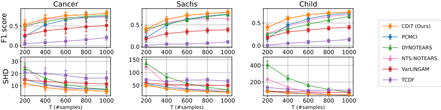
Performance vs. sample size. The results are illustrated in Fig. 2. As shown in the figure, the performance of all methods gets better as the sample size increases, while degrades as the data dimension increases. CDiT achieves the best performance in most cases except for Cancer network, where the SHD of CDiT and PCMCI are very close. Another competitive method is NTS-NOTEARS, whose F1 score approaches that of PCMCI when the sample size increases. However, there remains a gap between them in terms of SHD. The primary reason is that NTS-NOTEARS predicts numerous false edges, resulting in low Precision (see Fig. 6 in Appendix). VarLiNGAM and TCDF are not competitive with the other methods, especially when the sample size is large. An advantage of CDiT is it performs relatively better with a limited number of samples.
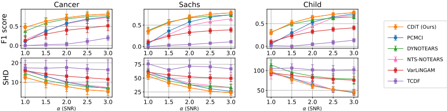
Performance vs. SNR. From Fig. 3 we can see that SNR highly affects the performance of all methods. All their performance improves as SNR increases. our method CDiT still achieves the best performance in most cases. These results are similar to those for different sample sizes, where CDiT, DYNOTEARS, NTS-NOTEARS and PCMCI are competitive, while the remaining two are not. And we can see that CDiT can handle low SNR cases better than the other methods.
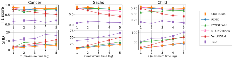
Performance vs. maximum time lag. The results are presented in Fig. 4. We can see the F1 scores of almost all methods are not significantly affected by the value of maximum time lag, except for VarLiNGAM, whose performance degrades obviously as the maximum time lag increases. On the other hand, the SHD of all methods gets larger with the maximum time lag increasing. The main reason is that the ground-truth window graph becomes denser when the maximum time lag increases. Among all methods, CDiT and PCMCI are better equipped to handle cases with multiple time lags. In most cases, CDiT obtains the best performance in terms of F1 score and SHD.
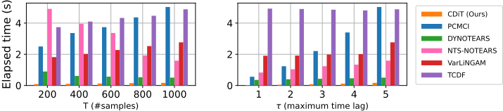
Elapsed time. As the time consumed by all methods is mainly dependent on the sample size and the maximum time lag, we fix SNR a to the default value 3 and only evaluate the performance on Child due to space limit. The results are shown in Fig. 5. It is worth noting that the elapsed time of PCMCI, NTS-NOTEARS and TCDF is divided by 10 for better visualization, as they are time-consuming. The time consumed by DYNOTEARS and NTS-NOTEARS decreases as the sample size increases, because fewer samples will lead to longer convergence time during iterations. In conclusion, CDiT runs significantly faster than all the other methods.
| CDiT (Ours) | PCMCI | DYNOTEARS | NTS-NOTEARS | VarLiNGAM | TCDF | ||
|---|---|---|---|---|---|---|---|
| Recall | 1.00 | 1.00 | 0.58 | 0.67 | 0.48 | 0.52 | |
| Precision | 0.60 | 0.27 | 0.59 | 0.69 | 0.47 | 0.68 | |
| NETSIM | F1 score | 0.75 | 0.42 | 0.58 | 0.68 | 0.48 | 0.59 |
| SHD | 22 | 90 | 27 | 22 | 35 | 24 | |
| Time (s) | 0.9 | 159.0 | 10.0 | 253.8 | 12.5 | 173.2 | |
| Recall | 0.18 | 0.36 | 0.00 | 0.27 | 0.27 | 0.00 | |
| Precision | 0.50 | 0.09 | 0.00 | 0.06 | 0.1 | 0.00 | |
| DREAM3 | F1 score | 0.27 | 0.14 | 0.00 | 0.09 | 0.15 | 0.00 |
| SHD | 11 | 49 | 27 | 58 | 35 | 12 | |
| Time (s) | 0.1 | 3.6 | 0.3 | 53.2 | 1.0 | 111.5 |
6.2 Results on Real Data
Here we evaluate CDiT with two real-world biological datasets NETSIM and DREAM3. These two datasets are often used to evaluate both summary and window causal graph discovery methods [Assaad et al., 2022; Gong et al., 2023]. NETSIM is an fMRI imaging dataset with 15 time series describing different regions in the brain with 200 timestamps representing the signal of each human subject. The goal is to infer the connectivity between different brain regions. It is generally assumed that different human subjects share the same connectivity. We use the data 1 from the 1∼20 subjects with self-connections, i.e., the dimension d = 15 and the total sample size T = 4000. DREAM3 [Prill et al., 2010] is a gene network dataset consisting of silico measurements of gene expression levels for the networks. We use the data from the first network having 10 time series and 80 timestamps without self-connection, i.e., d = 10 and T = 80. The goal is to recover the actual network structure with such a few samples. The maximum time lag for each method is fixed at τ = 5 on both two datasets.
The results are presented in Tab. 1. CDiT achieves much better performance on the two datasets than the other methods in terms of F1, SHD and elapsed time. DYNOTEARS, NTS-NOTEARS, VarLiNGAM and TCDF also get competitive accuracy while PCMCI achieves the best Recall but very low Precision.We also see that PCMCI, NTS-NOTEARS and TCDF are time-consuming when the sample size is large, which is consistent with the results shown in Fig. 5. On the other hand, the performance of all the methods degrades on DREAM3. One major reason is the small sample size of 80, which leads to 0% accuracy for DYNOTEARS and TCDF. However, our method can still cope with such hard cases causing many Type-II errors, resulting in low Recall.
1 https://www.fmrib.ox.ac.uk/datasets/netsim/index.html
7 Conclusion
In this work, we develop a constraint-based window causal graph discovery method in time series with multiple time lags. A significant advantage of our method is its efficiency, having a time complexity of O(d 2 TCI) where d is the number of sub-series, TCI is the time complexity of the chosen CI test. We conduct extensive experiments with performance comparison to typical existing methods, including Granger causality, constraint-based and score-based methods. We show in simulations that our method can handle the cases of fewer samples and low SNR better than the other competitors with only 1/3 ∼ 1/1000 of their consuming time. Furthermore, the results on two well-known real-world biological datasets also indicate that our method outperforms the other methods. Currently, the proposed method struggles with cases involving latent confounders or contemporaneous links, which requires additional CI tests to achieve it. We leave this for future work.
Acknowledgements
This work was supported by National Natural Science Foundation (62372116 and 62472415) and Guangdong Basic and Applied Basic Research Foundation (2025A1515010103).
Contribution Statement
Yewei Xia and Yixin Ren contributed equally to this work. Corresponding authors: Hao Zhang, Shuigeng Zhou.
@inproceedings{ijcai2025p1011,
  title     = {Efficient Constraint-based Window Causal Graph Discovery in Time Series with Multiple Time Lags},
  author    = {Xia, Yewei and Ren, Yixin and Cheng, Hong and Zhang, Hao and Guan, Jihong and Xu, Minchuan and Zhou, Shuigeng},
  booktitle = {Proceedings of the Thirty-Fourth International Joint Conference on
               Artificial Intelligence, {IJCAI-25}},
  publisher = {International Joint Conferences on Artificial Intelligence Organization},
  editor    = {James Kwok},
  pages     = {9095--9103},
  year      = {2025},
  month     = {8},
  note      = {Main Track},
  doi       = {10.24963/ijcai.2025/1011},
  url       = {https://doi.org/10.24963/ijcai.2025/1011},
}
TY - CPAPER TI - Efficient Constraint-based Window Causal Graph Discovery in Time Series with Multiple Time Lags AU - Xia, Yewei AU - Ren, Yixin AU - Cheng, Hong AU - Zhang, Hao AU - Guan, Jihong AU - Xu, Minchuan AU - Zhou, Shuigeng T2 - Proceedings of the Thirty-Fourth International Joint Conference on Artificial Intelligence, IJCAI-25 PB - International Joint Conferences on Artificial Intelligence Organization PY - 2025 SP - 9095 EP - 9103 DO - 10.24963/ijcai.2025/1011 UR - https://doi.org/10.24963/ijcai.2025/1011 ER -Copied
Machine-readable versions of this paper, for tools and AI agents:





