
Conditional Independent Test in the Presence of Measurement Error with Causal Structure Learning
Proceedings of the Thirty-Fourth International Joint Conference on Artificial Intelligence. Main Track. Pages 9112-9120.
https://doi.org/10.24963/ijcai.2025/1013
Keywords
- Uncertainty in AI: UAI: Bayesian networks
- Uncertainty in AI: UAI: Causality, structural causal models and causal inference
- Machine Learning: ML: Causality
- Uncertainty in AI: UAI: Graphical models
Abstract
Testing conditional independence is a critical task, particularly in causal discovery and learning in Bayesian networks. However, in many real-world scenarios, variables are often measured with errors, such as those introduced by insufficient measurement accuracy, complicating the testing process. This paper focuses on testing conditional independence in the linear non-Gaussian measurement error model, under the condition that measurement error noise follows a Gaussian distribution. By leveraging high-order cumulants, we derive rank constraints on the cumulant matrix and establish their role in effectively assessing conditional independence, even in the presence of measurement errors. Based on these theoretical results, we leverage the rank constraints of the cumulant matrix as a tool for conditional independence testing and incorporate it into the PC algorithm, resulting in the PC-ME algorithm — a method designed to learn causal structures from observed data while accounting for measurement errors. Experimental results demonstrate that the proposed method outperforms existing approaches, particularly in cases other methods encounter difficulties.
- [Baba et al., 2004] Kunihiro Baba, Ritei Shibata, and Masaaki Sibuya. Partial correlation and conditional cor- relation as measures of conditional independence. Aus- tralian & New Zealand Journal of Statistics, 46(4):657- 664, 2004.
- [Bouezmarni and Taamouti, 2014] Taoufik Bouezmarni and Abderrahim Taamouti. Nonparametric tests for condi- tional independence using conditional distributions. Jour- nal of Nonparametric Statistics, 26(4):697-719, 2014.
- [Chen et al., 2022] Zhengming Chen, Feng Xie, Jie Qiao, Zhifeng Hao, Kun Zhang, and Ruichu Cai. Identification of linear latent variable model with arbitrary distribution. In Proceedings 36th AAAI Conference on Artificial Intelli- gence (AAAI), 2022.
- [Chen et al., 2023] Zhengming Chen, Feng Xie, Jie Qiao, Zhifeng Hao, and Ruichu Cai. Some general identification results for linear latent hierarchical causal structure. In Proceedings of the Thirty-Second International Joint Con- ference on Artificial Intelligence, pages 3568-3576, 2023. IJCAI
- [Chen et al., 2024] Zhengming Chen, Jie Qiao, Feng Xie, Ruichu Cai, Zhifeng Hao, and Keli Zhang. Testing condi- tional independence between latent variables by indepen- dence residuals. IEEE Transactions on Neural Networks and Learning Systems, 2024.
- [Cui et al., 2018] Ruifei Cui, Perry Groot, Moritz Schauer, and Tom Heskes. Learning the causal structure of cop- ula models with latent variables. In Proceedings of the Thirty-Fourth Conference on Uncertainty in Artificial In- telligence, UAI 2018, pages 188-197. AUAI Press, 2018.
- [Dai et al., 2022] Haoyue Dai, Peter Spirtes, and Kun Zhang. Independence testing-based approach to causal discovery under measurement error and linear non-gaussian mod- els. Advances in Neural Information Processing Systems, 35:27524-27536, 2022.
- [Doran et al., 2014] Gary Doran, Krikamol Muandet, Kun Zhang, and Bernhard Schölkopf. A permutation-based kernel conditional independence test. In UAI, pages 132- 141, 2014.
- [Fuller, 2009] Wayne A Fuller. Measurement error models. John Wiley & Sons, 2009.
- [Huang et al., 2022] Biwei Huang, Charles Jia Han Low, Feng Xie, Clark Glymour, and Kun Zhang. Latent hier- archical causal structure discovery with rank constraints. In Advances in Neural Information Processing Systems, 2022.
- [Jin et al., 2024] Songyao Jin, Feng Xie, Guangyi Chen, Bi- wei Huang, Zhengming Chen, Xinshuai Dong, and Kun Zhang. Structural estimation of partially observed linear non-gaussian acyclic model: A practical approach with identifiability. In ICLR, 2024.
- [Kalisch and Bühlman, 2007] Markus Kalisch and Peter Bühlman. Estimating high-dimensional directed acyclic graphs with the pc-algorithm. Journal of Machine Learn- ing Research, 8(3), 2007.
- [Kelly, 2007] Brandon C Kelly. Some aspects of measure- ment error in linear regression of astronomical data. The Astrophysical Journal, 665(2):1489, 2007.
- [Lundborg et al., 2022] Anton Rask Lundborg, Rajen D Shah, and Jonas Peters. Conditional independence test- ing in hilbert spaces with applications to functional data analysis. Journal of the Royal Statistical Society Series B: Statistical Methodology, 84(5):1821-1850, 2022.
- [Meek, 1995] Christopher Meek. Causal inference and causal explanation with background knowledge. In UAI, pages 403-410, 1995.
- [Robin and Smith, 2000] Jean-Marc Robin and Richard J Smith. Tests of rank. Econometric Theory, 16(2):151- 175, 2000.
- [Schkoda and Drton, 2023] Daniela Schkoda and Mathias Drton. Goodness-of-fit tests for linear non-gaussian struc- tural equation models. arXiv preprint arXiv:2311.04585, 2023.
- [Silva et al., 2006] Ricardo Silva, Richard Scheine, Clark Glymour, and Peter Spirtes. Learning the structure of lin- ear latent variable models. JMLR, 7(Feb):191-246, 2006.
- [Spirtes and Glymour, 1991] Peter Spirtes and Clark Gly- mour. An algorithm for fast recovery of sparse causal graphs. Social science computer review, 9(1):62-72, 1991.
- [Spirtes et al., 2000] Peter Spirtes, Clark Glymour, and Richard Scheines. Causation, Prediction, and Search. MIT press, 2000.
- [Spirtes, 2013] Peter Spirtes. Calculation of entailed rank constraints in partially non-linear and cyclic models. In UAI, pages 606-615. AUAI Press, 2013.
- [Sullivant et al., 2010] Seth Sullivant, Kelli Talaska, Jan Draisma, et al. Trek separation for gaussian graphical models. The Annals of Statistics, 38(3):1665-1685, 2010.
- [Totton and White, 2011] Nicola Totton and Paul White. The ubiquitous mythical normal distribution. Research and In- novation, 1:1-23, 2011.
- [Watson and Wright, 2021] David S Watson and Marvin N Wright. Testing conditional independence in supervised learning algorithms. Machine Learning, 110(8):2107- 2129, 2021.
- [Xie et al., 2022] Feng Xie, Biwei Huang, Zhengming Chen, Yangbo He, Zhi Geng, and Kun Zhang. Identification of linear non-gaussian latent hierarchical structure. In Inter- national Conference on Machine Learning, pages 24370- 24387. PMLR, 2022.
- [Xie et al., 2023] Feng Xie, Yan Zeng, Zhengming Chen, Yangbo He, Zhi Geng, and Kun Zhang. Causal discovery of 1-factor measurement models in linear latent variable models with arbitrary noise distributions. Neurocomput- ing, 2023.
- [Xie et al., 2024] Feng Xie, Biwei Huang, Zhengming Chen, Ruichu Cai, Clark Glymour, Zhi Geng, and Kun Zhang. Generalized independent noise condition for estimating causal structure with latent variables. Journal of Machine Learning Research, 25(191):1-61, 2024.
- [Yang et al., 2022] Yuqin Yang, AmirEmad Ghassami, Mo- hamed Nafea, Negar Kiyavash, Kun Zhang, and Ilya Sh- pitser. Causal discovery in linear latent variable models subject to measurement error. Advances in Neural Infor- mation Processing Systems, 35:874-886, 2022.
- [Zhang et al., 2011] Kun Zhang, Jonas Peters, Dominik Janzing, and Bernhard Schölkopf. Kernel-based condi- tional independence test and application in causal discov- ery. In Proceedings of the Twenty-Seventh Conference on Uncertainty in Artificial Intelligence, pages 804-813, 2011.
- [Zhang et al., 2018] Kun Zhang, Mingming Gong, Joseph D Ramsey, Kayhan Batmanghelich, Peter Spirtes, and Clark Glymour. Causal discovery with linear non-gaussian mod- els under measurement error: Structural identifiability re- sults. In UAI, pages 1063-1072, 2018.
- [Zhang et al., 2019] Hao Zhang, Shuigeng Zhou, Jihong Guan, and Jun Huan. Measuring conditional independence by independent residuals for causal discovery. ACM Trans- actions on Intelligent Systems and Technology (TIST), 10(5):1-19, 2019.
- [Zhang et al., 2022] Hao Zhang, Shuigeng Zhou, Kun Zhang, and Jihong Guan. Residual similarity based condi- tional independence test and its application in causal dis- covery. In Proceedings of the AAAI conference on artificial intelligence, volume 36, pages 5942-5949, 2022.
- [Zhou et al., 2020] Yeqing Zhou, Jingyuan Liu, and Liping Zhu. Test for conditional independence with application to conditional screening. Journal of Multivariate Analysis, 175:104557, 2020.
References were extracted automatically from the PDF and may contain errors.
Full text extracted automatically from the PDF; figures, tables and equations may differ. The PDF is the version of record.
1 Introduction
The conditional independence (CI) test aims to assess whether a correlation relation exists between two variables when conditioned on a set of other variables. It has been broadly applied across various fields like statistics, machine learning, and causal discovery [Zhou et al., 2020; Watson and Wright, 2021; Bouezmarni and Taamouti, 2014; Lundborg et al., 2022; Spirtes et al., 2000].
When the data model is presumed to be linear, the partial correlation test [Baba et al., 2004] is a well-known and effective tool for examining conditional independence relations among variables. Specifically, let Xi and Xj be two random variables and Xp be a vector, if the CI relation between Xi and Xj given Xp holds, i.e., Xi ⫫ Xk∣Xp, the partial correlation coefficient would be zero, denoted by ρXiXj .Xp = 0. Thus, one can examine whether the partial correlation coefficient is zero to discover the CI relations among observed variables. Obtaining these CI relations usually can be used to improve downstream tasks, such as constructing causal structures over observed variables, where the CI relations correspond to d-separation in the causal graphical model [Spirtes and Glymour, 1991; Spirtes et al., 2000].
∗Corresponding author.
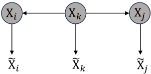
However, due to uncertainties in the real environment, the variable of interest is often difficult to measure directly and instead collected under the existence of measurement errors [Totton and White, 2011; Fuller, 2009; Kelly, 2007]. An example of measurement error is depicted in Fig. 1, where Xi, Xj, and Xk represent hidden variables of interest. When there exists some disturbing noise that directly causes the observed variable, one can only observe the variables ˜ Xi, ˜ Xj , and ˜ Xk (known as measured variables). Since the CI relations only hold on Xi ⫫ Xj∣Xk, in this case, the partial correlation coefficient ρ ˜ Xi ˜ Xj. ˜ Xk ≠ 0, implying the CI relations of Xi ⫫ Xj∣Xk can not be tested from ˜ Xi, ˜ Xj, and ˜ Xk (further details can be found in Example 2). Such a problem will lead to uninformative relations discovery or incorrect causal structure learning. Therefore, it is necessary to investigate how to learn the CI relations among hidden variables only from their measured variables.
Measurement error has been a topic of increasing interest in causal discovery. For instance, [Zhang et al., 2018] introduces a method for inferring causal structures in the presence of measurement error by leveraging non-Gaussianity, showing that the causal structure can be identified up to an ancestral ordered grouping (AOG) equivalence class. Similarly, [Yang et al., 2022] exploits the sparsity of the mixing matrix to propose a method for identifying linear latent variable models affected by measurement error. These identifiability results mainly rely on overcomplete independent component analysis (ICA), which, despite its theoretical appeal, often encounters computational challenges and risks convergence to local optima. Recently, [Dai et al., 2022] introduced the TIN condition to capture causal structure patterns in linear non-Gaussian models, proving that the partially causal order can be identified even in the presence of measurement error. While this approach effectively verifies d-separation relations (i.e., conditional independence) among hidden variables, it imposes structural constraints, such as the requirement that each hidden variable must have at least two observed variables as children. This assumption significantly restricts the applicability of the TIN condition in scenarios involving measurement error. Overall, existing methods struggle to efficiently identify conditional independence (CI) relations among latent variables solely from the observed variables without imposing additional assumptions. As shown in Fig. 1, for instance, existing methods may fail to effectively test the Xi ⫫ Xj ∣Xk by only using measured variables ˜ Xi, ˜ Xj and ˜ Xk .
In this paper, we address the problem of testing conditional independence (CI) relations among hidden variables only from their measured variables, under the linear nonGaussian measurement error model. We find out a sufficient condition-namely, the partial Gaussian noise assumption, where the noise term of the observed variables follows a Gaussian distribution-that enables the identification of dseparation relations from the high-order statistics of the hidden variables. Specifically, we first establish an equivalence between partial correlation and the rank deficiency of the correlation coefficient matrix. We then prove that rank constraints on the covariance matrix can be generalized to the higher-order cumulant matrix, enabling the identification of d-separation relations among latent variables. Based on this theoretical result, we propose a structure learning algorithm, the PC-ME algorithm, to infer causal structures among latent variables from their measured variables. Furthermore, we show that the PC-ME algorithm can identify the causal structure up to a Markov equivalence class.
Our contributions are summarised as follows:
- We generalize partial correlation to the case of measurement error and study the properties of rank deficiency of the higher-order cumulant matrix, under the linear nonGaussian measurement model and the partial Gaussian noise assumption.
- We propose an efficient algorithm to infer causal structures among hidden variables up to a Markov equivalence class by leveraging the properties of rank deficiency in the higher-order cumulant matrix.
- We empirically demonstrate that the proposed algorithm can asymptotically recover the correct causal structure under mild assumptions.
2 Linear Non-GaussianMeasurement Error Model
In this paper, we focus on the problem of testing conditional independence in the presence of measurement error, specifically within the framework of linear non-Gaussian models. Our theoretical results are built upon causal graphical models. In a causal graph, we use Pa(Vi) = {Vj∣Vj → Vi}, Ch(Vi) = {Vj∣Vi → Vj} to denote the set of parents and children of Vi, respectively. Due to space limitation, some graphical notations, such as d-separation and V-structure, are used here without explicit definitions, which can be found in the standard literature [Spirtes et al., 2000].
We start with the definition of the linear non-Gaussian model. Let X = {X1,⋯,Xn} denote the variable set of interest, in the linear non-Gaussian model, the data generation process for Xi ∈ X is given by the following equation:
where PaXi is the parent set of Xi, bij is the causal effect fromXj to Xi, and ni represents noise terms of Xi that follows non-Gaussian distribution. Without loss of generality, we assume all noise terms are independent of each other and the mean of noise is zero.
In real-world scenarios, variables of interest are often difficult to observe directly (commonly referred to as unobserved or hidden variables) and are instead measured with additive measurement error. To formalize the existence of measurement error, we present the linear non-Gaussian Measurement error Model (LiNGMME) as follows.
Definition 1 (LiNGMME). Let X be the hidden variable of interest that follows the linear non-Gaussian model, and ˜Xbe the measured variable set of X, we say ˜X follows the LiNGMME model if for ˜ Xi, ˜ Xi ∈ ˜X, it is generated by:
where Xi ∈ X is hidden variable, βXi→ ˜ Xi is disturbing strength fromXi to ˜ Xi, and ei are measurement error term.
Recently, the linear non-Gaussian model with measurement error has been extensively studied, such as [Yang et al., 2022; Zhang et al., 2018; Dai et al., 2022]. These works usually assume that all noise term, including those associated with hidden variables and measured variables, follow a non-Gaussian distribution. Under this assumption, the causal structure can be identified up to an Ancestral Ordered Grouping (AOG) equivalence class [Zhang et al., 2018]. In this paper, we explore a different condition where the noise term of the measured variables follows a Gaussian distribution, which enables the identifiability of conditional independence relations among hidden variables.
Condition 1 (Partial GaussianCondition). In LiNGMME, the noise term of the measured variable ei follows a Gaussian distribution.
In general, Condition 1 is reasonable and holds in most cases, as the Gaussian distribution is ubiquitous and commonly observed in many real-world scenarios, as discussed in [Totton and White, 2011; Fuller, 2009; Kelly, 2007].
Objective. In this paper, assuming Condition 1 holds, our goal is to investigate how to identify the conditional independence (CI) relations among hidden variables X only using their measured variables ˜X, under the LiNGAMME.
3 Conditional Independence Test Under Measurement Error
To achieve our goal, in this section, we provide an algebraic solution for identifying the conditional independence (CI) relations among hidden variables. First, we revisit partial correlation testing, a well-known method for testing CI, and explain why it fails in the presence of measurement error (Sec. 3.1). Next, we derive an equivalent expression for partial correlation from an algebraic perspective, specifically through the rank deficiency of the covariance matrix, and demonstrate how this can be extended to rank constraints on the higherorder cumulant matrix. By exploring these properties, we prove that the CI relations among latent variables can be identified (Sec. 3.2).
3.1 Partial Correlation Test
In a linear model, such as the linear Gaussian model (i.e., noise term follow Gaussian distribution in Eq. (1)), partial correlation is a commonly used tool for testing conditional independence, and is specifically defined as follows:
Definition 2 (Partial Correlation). The partial correlation coefficient of random variables Xi and Xj given Xp, is de-
where ρXiXj , ρXiXp , and ρXjXp represent the correlation coefficients of Xi and Xj, Xi and Xp, Xj and Xp, respectively
Specifically, CI relations can be examined by checking whether the partial correlation coefficient is zero. For instance, consider the structure in Fig. 1, where the CI relation Xi ⫫ Xj∣Xk holds. This can be tested by checking whether the partial correlation coefficient ρXiXj⋅Xk is zero. However, in the presence of measurement error, only ˜Xi, ˜Xj and ˜Xk are observed. In this case, the partial correlation test cannot reliably identify the CI relations among the latent variables Xi and Xj . Next, we give an example to illustrate this.
Illustrative Example
Consider the graph in Fig. 1, where Xi, Xj and Xk are hidden variables and ˜ Xi, ˜ Xj, and ˜ Xk are observed variables that are measured with measurement error. According to the definition of LiNGAMME, the data generation processes are
To construct the CI test using partial correlation, it is sufficient to check whether the numerator is zero. Specifically, each term of the numerator of the partial correlation coefficient between ˜ Xi and ˜ Xj given ˜ Xk is as follows.
Without loss of generality, assume that all observed variables are standardized, i.e., have unit variance. If the numerator of the partial correlation coefficient is zero, then we have
which does not hold in most cases. Note that if the above holds, it implies that either no measurement error exists or the measurement error can be ignored. There are two factors that prevent the partial correlation test from working: one is the disturbing strength from Xk to ˜Xk, and the other is the measurement error noise ek (or, ˜Xk). Generally speaking, without further constraints, the partial correlation test cannot be used in the presence of measurement error.
3.2 Rank Deficiency of High-order Cumulants Matrix
The above example illustrates why partial correlation does not work in the presence of measurement error: there exists disturbing strength βXk→ ˜Xk and an additional noise term ek, which causes the vanishing test to fail. To tackle this issue, fortunately, we have found that these unexpected influences can be mitigated under Condition 1, by appropriately utilizing the properties of higher-order cross-cumulants.
Before introducing the main result, we first provide an equivalent representation of partial correlation from the algebraic perspective, used as the building block for later results. We begin with the following example.
Example 1 (Equivalent representation of partial correlation). Consider the graph in Fig. 1, where the CI relationship Xi ⫫ Xj∣Xk holds. This CI relation can be tested by checking whether the partial correlation coefficient ρXiXj⋅Xk is zero, i.e., ρXiXj - ρXiXk ⋅ ρXkXj = 0 holds. Without loss generality, assume Xi,Xj and Xk are all standardized, so that ρXkXk = 1. The vanishing of the partial correlation can then be rewritten as:
Such an equality can be transferred to the determinant of the correlation coefficient matrix between {Xi,Xk} and {Xj,Xk}, as shown below:
which means that the correlation coefficient matrix is not full rank, i.e., rank deficiency.
In our work, we refer to this algebraic property as a "rank constraint," following the terminology used in the original literature [Sullivant et al., 2010; Huang et al., 2022]. We further present the following lemma to establish the connection between the CI relation and the rank constraints of the coefficient matrix. In other words, the relationship between partial correlation and the rank deficiency of the coefficient matrix.
Lemma 1 (Rank constraints of covariance matrix [Sullivant et al., 2010]). AssumeXi,Xj andXp follow the linear Gaussian model, and let Y = (Xi, Xp) and Z = (Xj , Xp) represent two vectors, then Xi ⫫Xj∣Xp if and only if the rank of correlation coefficient matrix between Y and Z is ∣Xp∣.
Lemma 1 provides an equivalent formalization of the partial correlation test, where the rank constraint of the covariance matrix between two vectors holds, with the intersection set of the two vectors serving as the conditional set in the CI relation. It is important to note that, when all variables are standardized, the rank constraints of the coefficient matrix are equivalent to those of the covariance matrix.
Recall the illustrative example in Sec 3.1. Let Y = { ˜Xi, ˜Xk} andZ = { ˜ Xj, ˜Xk}, assuming all variables are standardized. In most cases, the correlation coefficient (covariance) matrix between Y and Z has full rank due to the influence of measurement error. Under Condition 1, the key idea to address this issue is the fact that the higher-order cross-cumulants of Gaussian noise are zero. Based on this observation, one may wonder whether the rank constraints of the covariance matrix can be extended to a higher-order cross-cumulants matrix, thereby removing the influence of the Gaussian noise term of the measured variables. Before delving into this fact, we first revisit the definition of cumulants and some fundamental properties.
Definition 3 (k-th order joint cumulant tensor). The kth order joint cumulant tensor of a random vector X = [X1, ...,Xn]T is the k-way tensor T (k) X inRn×⋯×n ≡ (Rn )k whose entry in (i1, ..., ik) is the joint cumulant:
where the sum is taken over all partitions (B1, . . . ,BL) of the multiset {i1, ..., ik}.
Remark 1. Consider k = 4, one can see that the four-order cumulant cum(Xi1 ,Xi2 ,Xi3 ,Xi4 ) is defined as
That is, the fourth-order cumulant is not equal to the fourth-order moment. Specifically, all non-fourth-order interaction terms are absent in the fourth-order cumulant.
One can see that the second-order cumulant is the covariance, and higher-order cumulants can be viewed as an extension of covariance, where certain properties, such as additivity, are preserved. This motivates us to further investigate the matrix of cross-cumulants, which corresponds to the 2D slice of the joint cumulant tensor.
Definition 4 (2D slice of joint cumulant tensor). For a random vector X with k-th order joint cumulant tensor T (k) X where k ≥ 2 and k is any even, denote its 2D matrix slice of k-th order joint cumulant tensor as C (k) , where
In particular, when k = 2, for a random vector X, C (2) X is the covariance matrix ΣX. Similar to Lemma 1, one can construct the cumulant matrix between two vectors Y and Z, as shown in the following example.
Example 2 (K-order cumulant matrix). For two vertices sets Z = {X1,X2,⋯,Xn},Y = {Xn+1,Xn+2,⋯,X2n}, let k ≥ 2, the k-order cumulant matrix between Z and Y is
Next, we will show that in the LiNGAMME, the CI relations among hidden variables can be tested by checking the rank constraints over the cumulant matrix of observed variables, as shown in Theorem 1.
Theorem 1 (Rank constraints of cumulant matrix). For hidden variables Xi, Xj, and a vector Xp, assume that their observed variables ˜ Xi, ˜ Xj, ˜ Xp follow the LiNGMME and any k-order cumulant among them exists. Let Y = { ˜ Xi, ˜ Xp} and Z = { ˜ Xj, ˜ Xp}. Then, under Condition 1, Xi ⊥⊥ Xj∣Xp generic hold if and only if the rank of k-order cumulant matrix between Z and Y is ∣Xp∣, i.e., Rank(C kY;Z) = ∣Xp∣.
Remark 2. One can see that Lemma 1 is a special case (when k = 2) of Theorem 1. The key difference is that, while CI relations cannot be identified using the rank of the covariance matrix, they can be tested by Theorem 1 under Condition 1.
We further provide an example to show how CI relations can be tested using the rank constraints of the cumulant matrix, even when the partial correlation test fails.
Example 3 (Testing CI relations using Theorem 1). Continuous the illustrative example in Sec. 3.1. Let Y = { ˜Xi, ˜Xk} and Z = { ˜Xj, ˜Xk}, assuming the 4-order cross-cumulant exists. Then the cumulants matrix between Y and Z is
where
One can see that C (4) Xi ,Xj C (4) Xk ,Xk - C (4) Xi ,Xk C (4) Xj,Xk = 0, which implies that the cumulant matrix C (4) Y;Z is rank deficiency, i.e., Rank(C (4) Y;Z) = 1. By Theorem 1, we can infer that Xi ⫫ Xj ∣Xk.
Intuitively, the reason why CI relations can be tested by checking the rank constraints of the cumulant matrix is that the cumulant matrix excludes any information from Gaussian measurement error noise due to the property that higher-order cumulants of Gaussian distributions are zero, e.g., E(e4k) = 0 in C (4) Xk,Xk . This result can be directly applied to the linear non-Gaussian causal model, providing an alternative method for CI testing.
Corollary 1 (Rank constraints in linear non-Gaussian model). Let Xi, Xj be two random variables and Xp be a vector in the linear non-Gaussian model. Suppose any korder cross-cumulant exists. Then, Xi ⊥⊥ Xj∣Xp generic holds if and only if the rank of any k-order cumulant matrix between vectors Y = (Xi, Xp) and vectors Z = (Xj , Xp) is ∣Xp∣, i.e., Rank(C kY;Z) = ∣Xp∣, where ∣Xp∣ are the dimension size of the vector.
In other words, Corollary 1 shows that if there is no measurement error, Lemma 1 generally holds and can be viewed as a special case of the rank constraints of the cumulant matrix, so that Rank(C 2Y,Z) = Rank(C kY,Z) with k ≥ 2. Practically, in the linear non-Gaussian model, one can enhance the statistical robustness of the CI test by summarizing the results across multiple k-order cumulants matrices.
Example 4. Let k = {4, 6, 8}, Y = { ˜Xi, ˜Xk} and Z = { ˜Xj, ˜Xk}. If we obtain results from observational data such that Rank(C (4) Y,Z) = 1, Rank(C (6) Y,Z) = 1, and Rank(C (8) Y,Z) = 2, we can infer that Xi ⫫ Xj∣Xk, because most of the results tend to support the rank deficiency of the cumulant matrix.
Moreover, in practice, an important problem is how to test the rank constraints of the cumulant matrix using empirical data. To address this, we propose the following hypothesis test.
Test the rank of Cumulant Matrix We test the rank of cumulant by leveraging CR statistic [Schkoda and Drton, 2023; Robin and Smith, 2000], which is formed to test the null hy-
where ˆ C be an asymptotically normal estimator of C and the null distribution of the CR statistic may be asymptotically approximated by a weighted sum of independent χ21 random variables, the weights being determined by the asymptotic covariance matrix of ˆ C.
4 Application to Causal Structure Learning
Conditional independence (CI) tests are widely used in causal discovery, where that the true causal structure of n random variables can be represented by a directed acyclic graph
(DAG) G. In this section, we apply the proposed CI testing tool to the causal discovery task, presenting an algorithm that can infer causal structures from observational data in the presence of measurement error. To ensure the asymptotic correctness of the causal discovery methods, some necessary causal assumptions are required.
Assumption 1 (Causal Markov condition). The joint distribution P satisfies all CIs that are imposed by the true causal graph (generating process of the data).
Assumption 2 (Rank Faithfulness [Spirtes, 2013]). Let a distribution P be (linearly) rank-faithful to a directed acyclic graph G if every rank-constraint on a sub-cumulants matrix that holds in P is entailed by every free-parameter linear structural model with path diagram equal to G.
Note that the causal Markov condition and faithfulness assumption are commonly used in the constraint-based causal discovery algorithm, such as PC algorithm [Spirtes et al., 2000]. Traditionally, the PC algorithm recovers the graph structure by leveraging the (conditional) independence relations identified in the data. However, it is well known that small mistakes early in the algorithm (e.g., failing to detect an independence relation) can propagate and lead to significant errors in the resulting DAG. Consequently, the performance of such methods heavily depends on the accuracy of the (conditional) independence testing procedures.
In the LiNGAMME framework, as shown in the illustrative example in Sec. 3.1, the conditional independence test becomes unreliable in the presence of measurement error, which can lead to incorrect results produced by the PC algorithm. To address this issue, by replacing the conditional independence test in the PC algorithm with our proposed tool, we present the PC algorithm with measurement error (abbreviated as PCME), as shown in Algorithm 1.
As shown in Algorithm 1, we adopt the standard framework of the PC algorithm to learn the causal structure from observed variables in the LiNGAMME framework. Specifically, we initialize the complete undirected graph G on the set of hidden variables X. Then, we iteratively check whether each pair of hidden variables, Xi and Xj, are conditionally independent given a set of hidden variables Xp. This is achieved by testing the rank constraint of the cumulant matrix among the observed variables. Formally, Xi ⫫ Xj ∣ Xp holds if and only if Rank(C kY;Z) = ∣Xp∣, where Y = { ˜Xi, ˜Xp} and Z = { ˜Xj, ˜Xp}. If Xi and Xj are conditionally independent given a conditional set, the edge between Xi and Xj in G is removed. By repeating this procedure, we obtain the skeleton of the hidden variables. Simultaneously, we record the corresponding CI test results, including the conditional set of Xi and Xj in the d-separated set Sepset(Xi,Xj), which is useful for inferring causal directions and reducing redundant tests in subsequent steps. Next, we orient the causal directions by detecting V-structures, i.e., checking whether a local structure Xi - Xk - Xj forms a V-structure. If it does, we orient it as Xi → Xk ← Xj. Finally, we apply Meek's rules [Meek, 1995] to infer additional causal directions and output a partial DAG (PDAG) of the hidden variables with respect to the observational data.
Algorithm 1 PC algorithm with measurement error (PC-ME)
Require: Observational dataset ˜X = { ˜ X1, . . . , ˜ Xm} Ensure: A partial DAG G.
Let ˜ Xi denote as its corresponding hidden variable Xi, Xi ∈ X;
Initialize the complete undirected graph G over the hidden variable set X;
for ∀Xi,Xj ∈ X and adjacent in G do
if ∃Xp ⊆ X \ {Xi,X)j} and (∣Xp∣ < k) such that Rank(C kY;Z) = ∣Xp∣ with Y = { ˜ Xi, ˜ Xp}, Z = { ˜ Xj, ˜ Xp} then
end if end for
for ∀Xi,Xj,Xk ∈ X such that the pair Xi, Xk and the pair Xj , X)k are adjacent in G but the pair Xi, Xj are not adjacent in G do
end if
end for
while at least one edge can be oriented do
if ∃Xi → Xj, Xj and Xk are adjacent, Xi and Xk are not adjacent and there is no arrowhead at Xj then orient Xj - Xk as Xj → Xk
end if
if ∃Xi and Xj, there is a directed path from Xi to Xj and an edge between Xi and Xj then orient Xi - Xj as Xi → Xj
end if
end while
Return a partial DAG of hidden variables;
Complexity analysis. The complexity of the PC-ME algorithm for a hidden variable causal structure graph G is bounded by the largest degree in G. Let k be the maximal degree of any vertex and let n be the number of vertices. Then in the worst case, the number of conditional independence tests among hidden variables required by the algorithm is bounded by
Since the PC-ME algorithm relies only on the constraints of conditional independence (CI), it generally identifies the causal structure only up to Markov equivalence classes, which are sets of graphs that represent exactly the same independences and CIs. Thus, we next give the identifiability results of the PC-ME algorithm.
Theorem 2 (The correctness of algorithm). Suppose the data generation process follows the LiNGAMME, and the causal Markov condition, rank faithfulness assumption, and Condition 1 hold. Given a sufficiently large sample size, the PC-ME algorithm asymptotically outputs the Markov equivalence classes of the hidden variables.
5 Simulation Experiments
In this section, we evaluate the practical performance of the proposed algorithm using synthetic data. First, we examine the performance in the CI test based on the rank constraints of cumulant matrices. Then, we verify the correctness of the PC-ME algorithm in the task of causal structure learning.
5.1 Performance of Conditional Independence Test
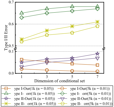
We conducted an experiment to verify the performance of the conditional independence test under the LiNGAMME. We consider the case whether Xi and Xj are conditional independence given by Xp, i.e., Xi ⫫ Xj∣Xp, where Xp = {X1, ..., Xm}. We adjust the dimension m of Xp to show that the proposed method is able to deal with the complexity case of conditional independent, ranging from 1 to 7. Specifically, we first generated the independent vector Xp, then Xi and Xi were generated as β⊺Xp + ε , where β is causal strength vector, which is generated uniformly in [-2, -0.5]∪[0.5, 2], ε is the noise term that follow the uniform distribution with U(-1, 1). Finally, we generate the observed variable according to the definition of LiNGAMME.
We compare our method with the partial correlation [Baba et al., 2004]- the well-known CI test method in linear models. We use Type I and Type II errors as evaluation metrics (for more details, refer to the appendix) to investigate how the size of the conditional set impacts performance. To see the performance of Type II, not all elements in Xp are the conditional set of Xi and Xj. We randomly select the independent variable into Xp with ranging 1 to 3. In our simulations, the sample size is fixed at [1000, 5000], and the significance level is set to [0.05, 0.01] for all methods.
The results are shown in Fig. 2, one can see that the probabilities of Type I errors closely align with the significance levels for our method, and meanwhile, the Type I error is close to significance level. These results show that our CI test tool can tackle the CI test under the existence of measurement error. Although with the increase in the dimensionality of Xp, the performance of our method noticeably decreases. This decrease is reasonable because the accuracy of the rank test decreases with the higher dimension matrix [Schkoda and Drton, 2023]. Furthermore, all of baseline methods exhibit poor performance in terms of Type I&II error, indicating the existing methods are not capable of handling the CI test in the presence of measurement error.
| Precision ↑ | F1 ↑ | ||||||
|---|---|---|---|---|---|---|---|
| Algorithm | Ours | PC | LPC | Ours | PC | LPC | |
| D=5 | 3k | 0.95 | 0.39 | 0.52 | 0.95 | 0.54 | 0.67 |
| 5k | 0.96 | 0.45 | 0.50 | 0.96 | 0.61 | 0.66 | |
| 10k | 0.96 | 0.43 | 0.51 | 0.97 | 0.59 | 0.66 | |
| D=10 | 3k | 0.92 | 0.42 | 0.51 | 0.93 | 0.58 | 0.66 |
| 5k | 0.95 | 0.43 | 0.46 | 0.95 | 0.59 | 0.62 | |
| 10k | 0.95 | 0.45 | 0.52 | 0.96 | 0.61 | 0.67 | |
| D=15 | 3k | 0.90 | 0.41 | 0.48 | 0.91 | 0.57 | 0.64 |
| 5k | 0.92 | 0.42 | 0.48 | 0.93 | 0.58 | 0.64 | |
| 10k | 0.93 | 0.47 | 0.51 | 0.94 | 0.63 | 0.67 | |
5.2 Performance of Causal Structure Learning
To evaluate the effectiveness of the proposed algorithm in causal structure learning, we employ the PC-ME algorithm on the random graph under the LiNGAMME model. We then compare its performance with that of the original PC algorithm, where CI relations are tested by partial correlation [Spirtes et al., 2000], and latent PC algorithm (abbreviated as LPC) [Chen et al., 2024], which allow to test the CI relations among hidden variables form measured variables.
Firstly, we construct the latent structure by randomly generating a Directed Acyclic Graph (DAG) [Kalisch and B¨uhlman, 2007], which can be represented as an n × n adjacency matrix, where n denotes the dimensionality of the latent variables. This matrix encodes the causal relationships among the hidden variables, with each element representing the causal strength between them. The hidden variable data is then generated from this DAG, with causal strength constrained to the interval [-2, -0.5] ∪ [0.5, 2], while the error term ni of each hidden variable Xi is sampled from either (i) a uniform distribution ni ∼ U(0.2, 1) (here four-order cumulant matrix is used in our method), or (ii) a standard exponential distribution. Subsequently, we generate observed variables corresponding to each hidden variable based on the definition of the LiNGAMEE. For instance, ˜ Xi = βXi→ ˜Xi Xi+ei, where ˜Xi is the observed variable of hidden variable Xi, βXi→ ˜Xi is disturbing strength, and ei is the corresponding noise term that follows the Gaussian distribution.
We simulate observational data under different settings and apply our algorithm along with baseline methods to these datasets. This allows us to assess how the performance varies across different scenarios. We control the following parameters: (1) varying the number of latent variables D = {5, 10, 15}, (2) adjusting the sample sizes {3k, 5k, 10k}. Additionally, we set the sparseness parameter when generating the DAG to s = 2/(k-1), where k represents the number of hidden variables, ensuring an average of two neighbors for each hidden variable [Cui et al., 2018]. Moreover, since the output of the PC algorithm is a partial DAG, we utilize precision, recall, and F1 score as metrics. In our analysis, the significance level of all methods is set to α = 0.01.
| Precision ↑ | F1 ↑ | ||||||
|---|---|---|---|---|---|---|---|
| Algorithm | Ours | PC | LPC | Ours | PC | LPC | |
| D=5 | 3k | 0.95 | 0.48 | 0.49 | 0.95 | 0.65 | 0.65 |
| 5k | 0.96 | 0.59 | 0.52 | 0.96 | 0.65 | 0.67 | |
| 10k | 0.97 | 0.55 | 0.54 | 0.97 | 0.70 | 0.68 | |
| D=10 | 3k | 0.93 | 0.50 | 0.51 | 0.94 | 0.66 | 0.66 |
| 5k | 0.95 | 0.48 | 0.47 | 0.95 | 0.65 | 0.63 | |
| 10k | 0.96 | 0.49 | 0.52 | 0.96 | 0.65 | 0.67 | |
| D=15 | 3k | 0.92 | 0.47 | 0.51 | 0.92 | 0.63 | 0.66 |
| 5k | 0.94 | 0.49 | 0.45 | 0.94 | 0.65 | 0.61 | |
| 10k | 0.95 | 0.52 | 0.53 | 0.95 | 0.67 | 0.68 | |
The experiment result of learning the causal skeleton is shown in Table 1 and Table 2. Our method outperforms all of the baseline methods, particularly in terms of precision and F1 score. This implies that the causal structure of the hidden variable estimated by our method is correct in most cases. Besides, one can see that all of the baseline methods exhibit poor F1 scores, indicating that existing methods are not able to handle scenarios involving measurement errors effectively. Due to space limitations, additional details on the experimental results are provided in the appendix.
6 RelatedWorks
Numerous methods exist for conditional independence (CI) testing and causal discovery with latent variables. For CI testing, there are the residual-based methods [Zhang et al., 2022; Zhang et al., 2019; Chen et al., 2024] and kernel-based approaches [Zhang et al., 2011; Doran et al., 2014]. For the task of causal discovery with latent variables, there are secondorder-based ones [Silva et al., 2006; Chen et al., 2022; Huang et al., 2022; Xie et al., 2023], higher-order statistics-based approaches [Xie et al., 2022; Xie et al., 2024; Jin et al., 2024; Chen et al., 2023]. While effective for CI testing and latent causal discovery, these methods do not account for measurement error, leaving a key gap in existing approaches.
7 Conclusion
We study the problem of testing conditional independence among observed variables in the presence of measurement error. In the LiNGAMEE model, by incorporating the higherorder cumulant, we present the rank constraint of the cumulant matrix, a novel CI tool capable of accommodating measurement errors. We further apply the proposed tool to the task of causal structure learning and present a practical algorithm PC-ME. The theoretical tool elegantly extends the application scope of partial correlation to account for measurement errors, and the proposed algorithm offers a solution for investigating and addressing measurement errors in the analysis. How to relax the model assumptions, e.g., allowing non-linear relations, would be interesting future directions.
Acknowledgements
This research was supported in part by the National Natural Science Foundation of China under grants No. 62476163 and U24A20233, and the Guangdong Basic and Applied Basic Research Foundation under grant number 2023B1515120020. We appreciate the comments from anonymous reviewers, which greatly helped to improve the paper.
@inproceedings{ijcai2025p1013,
  title     = {Conditional Independent Test in the Presence of Measurement Error with Causal Structure Learning},
  author    = {Zhang, Hongbin and Chen, Kezhou and Lin, Nankai and Yang, Aimin and Hao, Zhifeng and Chen, Zhengming},
  booktitle = {Proceedings of the Thirty-Fourth International Joint Conference on
               Artificial Intelligence, {IJCAI-25}},
  publisher = {International Joint Conferences on Artificial Intelligence Organization},
  editor    = {James Kwok},
  pages     = {9112--9120},
  year      = {2025},
  month     = {8},
  note      = {Main Track},
  doi       = {10.24963/ijcai.2025/1013},
  url       = {https://doi.org/10.24963/ijcai.2025/1013},
}
TY - CPAPER TI - Conditional Independent Test in the Presence of Measurement Error with Causal Structure Learning AU - Zhang, Hongbin AU - Chen, Kezhou AU - Lin, Nankai AU - Yang, Aimin AU - Hao, Zhifeng AU - Chen, Zhengming T2 - Proceedings of the Thirty-Fourth International Joint Conference on Artificial Intelligence, IJCAI-25 PB - International Joint Conferences on Artificial Intelligence Organization PY - 2025 SP - 9112 EP - 9120 DO - 10.24963/ijcai.2025/1013 UR - https://doi.org/10.24963/ijcai.2025/1013 ER -Copied
Machine-readable versions of this paper, for tools and AI agents:





