
ImputeINR: Time Series Imputation via Implicit Neural Representations for Disease Diagnosis with Missing Data
Proceedings of the Thirty-Fourth International Joint Conference on Artificial Intelligence. AI4Tech: AI Enabling Technologies. Pages 9241-9249.
https://doi.org/10.24963/ijcai.2025/1027
Keywords
- Advanced AI4Tech: Data-driven AI4Tech
- Domain-specific AI4Tech: AI4Care and AI4Health
Abstract
Healthcare data frequently contain a substantial proportion of missing values, necessitating effective time series imputation to support downstream disease diagnosis tasks. However, existing imputation methods focus on discrete data points and are unable to effectively model sparse data, resulting in particularly poor performance for imputing substantial missing values. In this paper, we propose a novel approach, ImputeINR, for time series imputation by employing implicit neural representations (INR) to learn continuous functions for time series. ImputeINR leverages the merits of INR in that the continuous functions are not coupled to sampling frequency and have infinite sampling frequency, allowing ImputeINR to generate fine-grained imputations even on extremely sparse observed values. Extensive experiments conducted on eight datasets with five ratios of masked values show the superior imputation performance of ImputeINR, especially for high missing ratios in time series data. We also validate that applying ImputeINR to impute missing values in healthcare data enhances the performance of downstream disease diagnosis tasks.
- [Afrifa-Yamoah et al., 2020] Eben Afrifa-Yamoah, Ute A Mueller, Stephen M Taylor, and Aiden J Fisher. Missing data imputation of high-resolution temporal climate time series data. Meteorological Applications, 27(1):e1873, 2020.
- [Alcaraz and Strodthoff, 2022] Juan Miguel Lopez Alcaraz and Nils Strodthoff. Diffusion-based time series impu- tation and forecasting with structured state space models. arXiv preprint arXiv:2208.09399, 2022.
- [Altman, 1992] Naomi S Altman. An introduction to ker- nel and nearest-neighbor nonparametric regression. The American Statistician, 46(3):175-185, 1992.
- [Cao et al., 2018] Wei Cao, Dong Wang, Jian Li, Hao Zhou, Lei Li, and Yitan Li. Brits: Bidirectional recurrent im- putation for time series. Advances in neural information processing systems, 31, 2018.
- [Chen and Wang, 2022] Yinbo Chen and Xiaolong Wang. Transformers as meta-learners for implicit neural repre- sentations. In European Conference on Computer Vision, pages 170-187. Springer, 2022.
- [Du et al., 2023] Wenjie Du, David Côté, and Yan Liu. Saits: Self-attention-based imputation for time series. Expert Systems with Applications, 219:119619, 2023.
- [Du, 2023] Wenjie Du. PyPOTS: a Python toolbox for data mining on Partially-Observed Time Series. arXiv preprint arXiv:2305.18811, 2023.
- [Fons et al., 2022] Elizabeth Fons, Alejandro Sztrajman, Yousef El-Laham, Alexandros Iosifidis, and Svitlana Vyetrenko. Hypertime: Implicit neural representation for time series. arXiv preprint arXiv:2208.05836, 2022.
- [Fung, 2006] David S Fung. Methods for the estimation of missing values in time series. 2006.
- [Guo et al., 2025] Jialong Guo, Ke Liu, Jiangchao Yao, Zhi- hua Wang, Jiajun Bu, Haishuai Wang, et al. Metan- erv: Meta neural representations for videos with spatial- temporal guidance. arXiv preprint arXiv:2501.02427, 2025.
- [Harutyunyan et al., 2019] Hrayr Harutyunyan, Hrant Khachatrian, David C. Kale, Greg Ver Steeg, and Aram Galstyan. Multitask learning and benchmarking with clinical time series data. Scientific Data, 6(1):96, 2019.
- [Institute, 2020] Max Planck Institute. Bgc jena: Weather station data. https://www.bgc-jena.mpg.de/wetter/, 2020. Accessed: 2025-05-27. Link
- [Jeong and Shin, 2022] Kyeong-Joong Jeong and Yong-Min Shin. Time-series anomaly detection with implicit neural representation. arXiv preprint arXiv:2201.11950, 2022.
- [Johnson et al., 2018] Alistair E W Johnson, David J Stone, Leo A Celi, and Tom J Pollard. The mimic code repos- itory: enabling reproducibility in critical care research. Journal of the American Medical Informatics Association, 25(1):32-39, 2018.
- [Kingma, 2014] Diederik P Kingma. Adam: A method for stochastic optimization. arXiv preprint arXiv:1412.6980, 2014.
- [Laboratory, 2006] National Renewable Energy Laboratory. Solar power data for integration studies. https://www.nrel. gov/grid/solar-power-data.html, 2006. Accessed: 2025- 05-27. Link
- [Lee et al., 2021] Jaeho Lee, Jihoon Tack, Namhoon Lee, and Jinwoo Shin. Meta-learning sparse implicit neural rep- resentations. Advances in Neural Information Processing Systems, 34:11769-11780, 2021.
- [Li et al., 2023a] Mengxuan Li, Peng Peng, Haiyue Sun, Min Wang, and Hongwei Wang. An order-invariant and interpretable dilated convolution neural network for chem- ical process fault detection and diagnosis. IEEE Transac- tions on Automation Science and Engineering, 2023.
- [Li et al., 2023b] Mengxuan Li, Peng Peng, Jingxin Zhang, Hongwei Wang, and Weiming Shen. Sccam: Supervised contrastive convolutional attention mechanism for ante- hoc interpretable fault diagnosis with limited fault sam- ples. IEEE Transactions on Neural Networks and Learn- ing Systems, 2023.
- [Li et al., 2024] Mengxuan Li, Ke Liu, Hongyang Chen, Jia- jun Bu, Hongwei Wang, and Haishuai Wang. Tsinr: Cap- turing temporal continuity via implicit neural representa- tions for time series anomaly detection. arXiv preprint arXiv:2411.11641, 2024.
- [Liu et al., 2023a] Ke Liu, Feng Liu, Haishuai Wang, Ning Ma, Jiajun Bu, and Bo Han. Partition speeds up learn- ing implicit neural representations based on exponential- increase hypothesis. In Proceedings of the IEEE/CVF In- ternational Conference on Computer Vision, pages 5474- 5483, 2023.
- [Liu et al., 2023b] Ke Liu, Ning Ma, Zhihua Wang, Jingjun Gu, Jiajun Bu, and Haishuai Wang. Implicit neural dis- tance optimization for mesh neural subdivision. In 2023 IEEE International Conference on Multimedia and Expo (ICME), pages 2039-2044. IEEE, 2023.
- [Liu et al., 2024] Yong Liu, Tengge Hu, Haoran Zhang, Haixu Wu, Shiyu Wang, Lintao Ma, and Mingsheng Long. itransformer: Inverted transformers are effective for time series forecasting. In The Twelfth International Confer- ence on Learning Representations, 2024.
- [Mai and Liu, 2022] Long Mai and Feng Liu. Motion- adjustable neural implicit video representation. In Pro- ceedings of the IEEE/CVF Conference on Computer Vision and Pattern Recognition, pages 10738-10747, 2022.
- [Molaei et al., 2023] Amirali Molaei, Amirhossein Amin- imehr, Armin Tavakoli, Amirhossein Kazerouni, Bobby Azad, Reza Azad, and Dorit Merhof. Implicit neural rep- resentation in medical imaging: A comparative survey. In Proceedings of the IEEE/CVF International Conference on Computer Vision, pages 2381-2391, 2023.
- [Naour et al., 2023] Etienne Le Naour, Louis Serrano, Léon Migus, Yuan Yin, Ghislain Agoua, Nicolas Baskio- tis, Patrick Gallinari, and Vincent Guigue. Time se- ries continuous modeling for imputation and forecast- ing with implicit neural representations. arXiv preprint arXiv:2306.05880, 2023.
- [Nie et al., 2024] Tong Nie, Guoyang Qin, Wei Ma, Yuewen Mei, and Jian Sun. Imputeformer: Low rankness-induced transformers for generalizable spatiotemporal imputation. In Proceedings of the 30th ACM SIGKDD Conference on Knowledge Discovery and Data Mining, pages 2260- 2271, 2024.
- [Repository, 2008] UCI Machine Learning Repository. Air quality data set. https://archive.ics.uci.edu/dataset/360/ air+quality, 2008. Accessed: 2025-05-27. Link
- [Reyna et al., 2019] MA Reyna, C Josef, R Jeter, SP Shashikumar, MB Westover, S Nemati, GD Clif- ford, and A Sharma. Early prediction of sepsis from clinical data: the physionetcomputing in cardiology challenge 2019. Critical Care Medicine, 48(2):210-217, 2019.
- [Saragadam et al., 2022] Vishwanath Saragadam, Jasper Tan, Guha Balakrishnan, Richard G Baraniuk, and Ashok Veeraraghavan. Miner: Multiscale implicit neural repre- sentation. In European Conference on Computer Vision, pages 318-333. Springer, 2022.
- [Schaffer et al., 2021] Andrea L Schaffer, Timothy A Dob- bins, and Sallie-Anne Pearson. Interrupted time series analysis using autoregressive integrated moving average (arima) models: a guide for evaluating large-scale health interventions. BMC medical research methodology, 21:1- 12, 2021.
- [Shan et al., 2023] Siyuan Shan, Yang Li, and Junier B Oliva. Nrtsi: Non-recurrent time series imputation. In ICASSP 2023-2023 IEEE International Conference on Acoustics, Speech and Signal Processing (ICASSP), pages 1-5. IEEE, 2023.
- [Silva et al., 2012] Ikaro Silva, George Moody, Daniel J Scott, Leo A Celi, and Roger G Mark. Predict- ing in-hospital mortality of icu patients: The phys- ionet/computing in cardiology challenge 2012. Computing in cardiology, 39:245, 2012.
- [Tashiro et al., 2021] Yusuke Tashiro, Jiaming Song, Yang Song, and Stefano Ermon. Csdi: Conditional score- based diffusion models for probabilistic time series impu- tation. Advances in Neural Information Processing Sys- tems, 34:24804-24816, 2021.
- [Van Buuren and Groothuis-Oudshoorn, 2011] Stef Van Bu- uren and Karin Groothuis-Oudshoorn. mice: Multivariate imputation by chained equations in r. Journal of statistical software, 45:1-67, 2011.
- [Wang et al., 2018] Haishuai Wang, Jia Wu, Peng Zhang, and Yixin Chen. Learning shapelet patterns from network- based time series. IEEE transactions on industrial infor- matics, 15(7):3864-3876, 2018.
- [Wang et al., 2024] Shiyu Wang, Haixu Wu, Xiaoming Shi, Tengge Hu, Huakun Luo, Lintao Ma, James Y Zhang, and JUN ZHOU. Timemixer: Decomposable multiscale mix- ing for time series forecasting. In The Twelfth Interna- tional Conference on Learning Representations, 2024.
- [Wu et al., 2023] Haixu Wu, Tengge Hu, Yong Liu, Hang Zhou, Jianmin Wang, and Mingsheng Long. Timesnet: Temporal 2d-variation modeling for general time series analysis. In The Eleventh International Conference on Learning Representations, 2023.
- [Yang et al., 2024] Yiying Yang, Fukun Yin, Wen Liu, Ji- ayuan Fan, Xin Chen, Gang Yu, and Tao Chen. Pm-inr: Prior-rich multi-modal implicit large-scale scene neural representation. In Proceedings of the AAAI Conference on Artificial Intelligence, volume 38, pages 6594-6602, 2024.
- [Yin et al., 2022] Fukun Yin, Wen Liu, Zilong Huang, Pei Cheng, Tao Chen, and Gang Yu. Coordinates are not lonely-codebook prior helps implicit neural 3d represen- tations. Advances in Neural Information Processing Sys- tems, 35:12705-12717, 2022.
- [Yoon et al., 2018] Jinsung Yoon, William R Zame, and Mi- haela van der Schaar. Estimating missing data in temporal data streams using multi-directional recurrent neural net- works. IEEE Transactions on Biomedical Engineering, 66(5):1477-1490, 2018.
- [Zeng et al., 2023] Ailing Zeng, Muxi Chen, Lei Zhang, and Qiang Xu. Are transformers effective for time series fore- casting? In Proceedings of the AAAI conference on artifi- cial intelligence, volume 37, pages 11121-11128, 2023.
- [Zhang et al., 2017] Shuyi Zhang, Bin Guo, Anlan Dong, Jing He, Ziping Xu, and Song Xi Chen. Cautionary tales on air-quality improvement in beijing. Proceedings of the Royal Society A: Mathematical, Physical and Engineering Sciences, 473, 2017.
- [Zhang et al., 2024] Shuyi Zhang, Ke Liu, Jingjun Gu, Xi- aoxu Cai, Zhihua Wang, Jiajun Bu, and Haishuai Wang. Attention beats linear for fast implicit neural representa- tion generation. In European Conference on Computer Vi- sion, pages 1-18. Springer, 2024.
- [Zhou et al., 2021] Haoyi Zhou, Shanghang Zhang, Jieqi Peng, Shuai Zhang, Jianxin Li, Hui Xiong, and Wan- cai Zhang. Informer: Beyond efficient transformer for long sequence time-series forecasting. In Proceedings of the AAAI conference on artificial intelligence, volume 35, pages 11106-11115, 2021.
- [Zhou et al., 2023] Tian Zhou, Peisong Niu, Liang Sun, Rong Jin, et al. One fits all: Power general time series analysis by pretrained lm. Advances in neural information processing systems, 36:43322-43355, 2023.
References were extracted automatically from the PDF and may contain errors.
Full text extracted automatically from the PDF; figures, tables and equations may differ. The PDF is the version of record.
1 Introduction
Healthcare data inherently exhibit a temporal structure, as they are often collected sequentially over time in the form of physiological signals, electronic health records, and clinical monitoring data, making time series analysis a fundamental approach for understanding and predicting healthrelated outcomes [Schaffer et al., 2021; Wang et al., 2018; Li et al., 2023a; Li et al., 2023b]. However, real-world healthcare data are frequently compromised by a substantial amount of missing values, which arise from various sources, such as sensor malfunctions, transmission errors, or irregular reporting intervals. The presence of missing values poses a significant challenge to disease diagnosis, as incomplete or corrupted data can distort model training and lead to unreliable predictions. Consequently, the imputation of missing data becomes a critical step in disease diagnosis. By filling in the gaps, imputation enables the restoration of a complete dataset, allowing diagnostic models to perform without the biases or inaccuracies that would otherwise result frommissing information.
∗Corresponding authors.
However, most existing imputation methods do not highlight the cases of extremely sparse observed values. These works assume that the proportion of masked values requiring imputation does not exceed 50%, which means that these methods still require a certain amount of known information. But in real-world healthcare data, the proportion of missing values is likely to be even higher. For example, the MIMIC-III dataset [Johnson et al., 2018], a public healthrelated database, contains 63.15% missing values. The PhysioNet 2012 and 2019 challenges [Silva et al., 2012; Reyna et al., 2019], which involved intensive care unit (ICU) patient data, reported a missing data rate of 79.67%, highlighting the prevalence of high missing rates in real-world healthcare datasets. Although some recent studies try to address imputation tasks in sparse scenarios [Alcaraz and Strodthoff, 2022; Tashiro et al., 2021], most work relies on diffusion-based methods, which involve the simulation of high-dimensional stochastic processes and multi-step iterative procedures. Consequently, these approaches are typically time-consuming and require a large number of training iterations, and their limited effectiveness in achieving accurate imputation can significantly impair the performance of downstream disease diagnosis tasks. How to perform imputation in extremely sparse scenarios remains challenging.
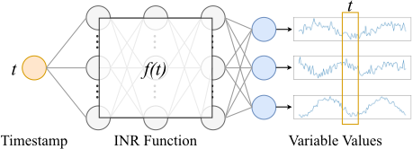
Recently, implicit neural representation (INR) has emerged as an effective method for continuously encoding diverse signals [Liu et al., 2023b; Molaei et al., 2023]. As shown in Figure 1, it learns continuous functions from discrete data points, mapping coordinates to signal values. By representing complex structures in a compact form, INR is not coupled to sampling frequency anymore, which allows for multi-sampling frequency inputs enabling effective feature extraction even with absent observed samples. Additionally, as a continuous function, INR has infinite sampling frequency, which means it can be queried at any coordinate. This capacity for infinite sampling frequency interpolation sets it apart from other imputation methods, making it a promising approach for finegrained imputation.
In this paper, we propose a novel time series imputation approach, named ImputeINR, which achieves effective imputation even in extremely sparse scenarios and the imputed data can further enhance the performance of downstream disease diagnosis tasks. Generally, we learn an INR continuous function for the target time series data and enable fine-grained interpolation with infinite sampling frequency. The parameters of the INR function are predicted by a transformerbased feed-forward network conditioned with sparsely observed values. More specifically, an adaptive group-based form of the INR function is proposed for capturing complex temporal patterns and cross-channel correlation features. It is a multilayer perceptron (MLP) composed of global layers and group layers. The former focuses on correlation information across all channels, while the latter emphasizes correlation information among variables within a single group. We observe that INR exhibits the strongest representational capacity when partitioning variables with similar distributions into the same group. Therefore, variable clustering is applied to determine the variable partition. Additionally, a multi-scale feature extraction module is incorporated to capture patterns at various temporal scales, achieving better fine-grained imputation. Experimentally, ImputeINR achieves state-of-theart performance on eight imputation benchmarks with various ratios of masked values. Moreover, we demonstrate that the imputed data with ImputeINR, compared to other methods, significantly improves the performance of downstream disease diagnosis tasks. The major contributions of this paper are summarized as follows:
- We propose ImputeINR, which learns INR continuous function to represent the continuous time series data. It achieves effective imputation in extremely sparse scenarios and the imputed data can improve the performance of downstream disease diagnosis tasks.
- We design an adaptive group-based form of the INR continuous function to effectively capture intricate temporal patterns and cross-channel correlation features.
- We apply variable clustering to determine the variable partition, allowing our group-based architecture to learn correlation information across all variables and among variables with similar distributions.
- Extensive experiments show that ImputeINR outperforms other baselines on eight datasets under five ratios of masked values. We also demonstrate that using ImputeINR for healthcare data imputation significantly enhances disease diagnosis performance.
2 RelatedWork
2.1 Time Series Imputation
The earliest time series imputation methods are based on the statistical properties of the data, using mean/median values or statistical models to fill in missing values, such as SimpleMean/SimpleMedian [Fung, 2006] and ARIMA [AfrifaYamoah et al., 2020]. Then, machine learning methods learn data patterns, showing greater adaptability and accuracy. Prominent works of these approaches include KNNI [Altman, 1992] and MICE [Van Buuren and Groothuis-Oudshoorn, 2011]. Although these methods are easy to interpret, their limitations lie in capturing the complex temporal and variable information inherent in time series data. Recently, there has been widespread interest in using deep models to capture complex temporal patterns for imputation of missing values, due to their powerful representation capabilities. Common architectures include RNN-based methods (e.g., M-RNN [Yoon et al., 2018], NRTSI [Shan et al., 2023], and BRITS [Cao et al., 2018]) , CNN-based methods (e.g., TimesNet [Wu et al., 2023]), MLP-based methods (e.g., DLinear [Zeng et al., 2023], TimeMixer [Wang et al., 2024]), transformer-based methods (e.g., SAITS [Du et al., 2023], FPT [Zhou et al., 2023], iTransformer [Liu et al., 2024], ImputeFormer [Nie et al., 2024]), diffusion-based methods (e.g., CSDI [Tashiro et al., 2021], SSSD [Alcaraz and Strodthoff, 2022]).
2.2 Implicit Neural Representations
INR uses neural networks to model signals as continuous functions rather than explicitly representing them as discrete points. It captures complex high-dimensional patterns in data by learning a continuous mapping from input coordinates to output values. Various scenarios have seen successful applications, such as 2D image generation [Saragadam et al., 2022; Liu et al., 2023a; Zhang et al., 2024], 3D scene reconstruction [Yin et al., 2022; Liu et al., 2023b; Yang et al., 2024], and video representations [Mai and Liu, 2022; Guo et al., 2025]. Since INR learns a continuous function, it is not coupled to the resolution, which implies that the memory needed to parameterize the signal does not depend on spatial resolution but rather increases with the complexity of the underlying signal. Also, INR has infinite resolution, which means it can be sampled at an arbitrary sampling frequency. Therefore, we leverage this characteristic of INR to perform time series imputation tasks. Sampling from the continuous function of INR enables fine-grained imputation even with extremely sparse observed data. To learn the INR for target signal, there are mainly two typical strategies: gradient-based meta-learning methods [Lee et al., 2021; Liu et al., 2023a] and feed-forward hyper-network prediction methods [Chen and Wang, 2022; Zhang et al., 2024]. In this work, we use a transformer-based feed-forward method to predict the INR for time series data since it can be easily adopted to an end-to-end imputation framework.
2.3 Implicit Neural Representations on Time Series Data
Several works have explored the use of INR to model time series data. INRAD [Jeong and Shin, 2022] leverages INR
to reconstruct time series data for anomaly detection. TSINR [Li et al., 2024] takes advantage of the spectral bias property of INR, prioritizing low-frequency signals and exhibiting reduced performance on high-frequency anomalous data to identify anomalies. However, these methods are specifically designed for anomaly detection tasks and are not suitable for imputation tasks. Currently, only a few works have attempted to leverage INR for time series imputation tasks, but each of these approaches has its own limitations. For example, HyperTime [Fons et al., 2022] utilizes INR to learn a compressed latent representation to capture the underlying patterns in time series for imputation and generation. However, it uses a permutation-invariant set encoder to extract features, leading to an insufficient representation of the underlying patterns in the time series. In addition, TimeFlow [Naour et al., 2023] utilizes continuous-time-dependent modeling and INR enhanced by a meta-learning-driven modulation mechanism for imputation and forecasting. However, treats each variable as an individual sample, thereby ignoring crucial intervariable correlations. Moreover, it fits the entire time series at once becoming computationally inefficient, particularly when dealing with long time series.
3 Methodology
3.1 ProblemFormulation
Imputation with Missing Data
Denote time series data with N variables and T timestamps as X = {x1, x2, . . . , xN} ∈ RN×T . The time series data X is incomplete and the mask rate is r ∈ [0, 1]. The corresponding binary mask matrix can be defined as M = {mn,t} ∈ {0, 1}N×T , where mn,t = 1 if xn,t is observed, and mn,t = 0 if xn,t is missing. The imputation task is to predict the missing values Xmiss such that the predicted values ˆX satisfy ˆX = Fθ(X,M), where Fθ mentions the model with parameters θ. The goal is to minimize the reconstruction error between the masked data and the imputed data:
where |Mmiss| is the total number of missing values in X and Xgt is the ground truth.
Disease Diagnosis
Let Ximputed represent the imputed version of X, where the missing values in X are imputed and the non-missing values in X are retained. The task is to utilize Ximputed for disease diagnosis, where a model G(·) is trained to predict disease labels ˆ y ∈ {0, 1} based on Ximputed:
where ˆ y = 0 denotes normal, and ˆ y = 1 indicates the presence of disease.
3.2 Method Overview
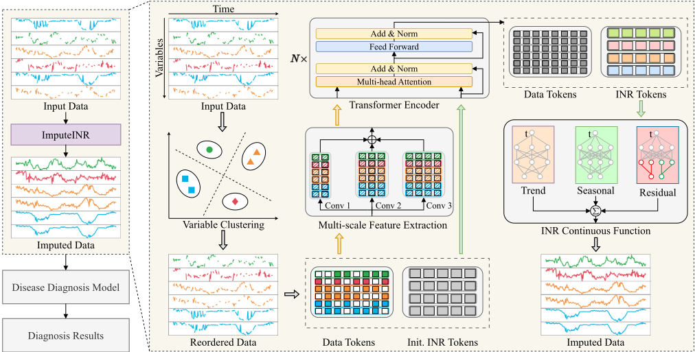
The core idea of ImputeINR is to leverage the inherent capability of INR to learn continuous functions, allowing for fine-grained imputation of time series data by querying at arbitrary timestamps. By leveraging this flexibility, ImputeINR can generate smooth and accurate estimates for missing data points, even with extremely sparse observed data. However, since time series data has inherently intricate temporal patterns and multi-variable properties, using a simple MLP as the INR continuous function to fit it is challenging. To address these issues, we design a novel form of INR continuous function specifically for time series data. Following the previous work [Fons et al., 2022; Li et al., 2024], this form includes three components to capture the trend, seasonal, and residual information to deal with the unique temporal patterns. Furthermore, to enhance the ability of ImputeINR to model multi-variable data, we propose an adaptive group-based architecture to learn complicated residual information. Each group focuses on variables with similar distributions. And we use a clustering algorithm to determine the variable partition. To further enhance the imputation capability of ImputeINR, we incorporate a multiscale module to capture information at different scales, improving fine-grained imputation performance.
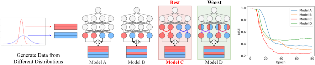
Figure 2 demonstrates the overall workflow of the proposed method. The masked data is first reordered based on the variable clustering results so that variables with similar distributions are placed adjacent to each other. This is to enable the subsequent representation of variables within the same cluster using the same group-based MLP in the INR continuous function. Then the reordered masked data is standardized and segmented into patches to prepare the data tokens. Simultaneously, we initialize the INR tokens, which are learnable vector parameters. The processed data tokens are input into convolutional layers of different scales to extract multi-scale features. Subsequently, these extracted features and the initialized INR tokens are fed together into the transformer encoder to predict the INR tokens. These INR tokens are essentially the parameters of the INR continuous function. Based on these parameters, the INR continuous function takes the timestamp t as input and predicts the masked values. Finally, the imputed data is then fed into the disease diagnosis model to obtain the diagnostic results.
3.3 Variable Clustering
We adopt a clustering algorithm C to cluster the variables of the time series data X ∈ RN×T based on the similarity matrix S ∈ RN×N , which partitions the variables into K clusters:
where Ck is a subset of the total variable set {x1, x2, . . . , xN} and its cardinality |Ck| denotes the number of variables in this cluster. The objective of the clustering function C is defined as follows:
where S(xi, xj) represents the similarity between variables xi and xj. Then we obtain the permutation matrix P ∈ RN×N :
where π is the permutation vector that orders the variables according to the clusters. Finally, the reordered matrix X′ with columns permuted according to π is given by:
In this reordered matrix X′ , rows (i.e., variables) are grouped according to the clusters.
3.4 Multi-scale Feature Extraction
To further capture features from different scales for finegrained imputation, the reordered data X′ ∈ RN×T is fed to multiple convolutional layers with varying scales. Each convolutional layer l refers to kernel size kl, stride sl, padding pl, and the number of output channels cl. For each output channel i in the lth convolutional layer, the convolution operation can be formulated as:
where W and b denote the weight matrix and bias matrix respectively. Then these features of different scales Φl (X′ ) ∈ Rcl×(T-kl+2pl+1) are concatenated to obtained the multiscale features ˙X ∈ R∑Ll=1 cl×(T ′-kl+2pl+1) . Finally, these features are fed to the transformer encoder together with the initialized INR tokens to predict the INR tokens.
3.5 INRContinuous Function
INR continuous function f maps the timestamp t to time series data:
where X(t) represents the output values of N variables at timestamp t. To effectively capture the complicated temporal patterns and successfully model the multiple variables, we design a novel form of INR continuous function. Following the previous work [Fons et al., 2022; Li et al., 2024], our INR continuous function includes three components to model trend, seasonal, and residual patterns separately. It can be defined as follows:
where t is the input timestamp and f(t) denotes the output (i.e., imputed data). The parameters in the INR continuous function are predicted by the transformer encoder (i.e., INR tokens).
Trend and Seasonal
The trend represents the long-termmovement or direction of the time series data. It is typically smooth and reflects gradual shifts in the level of the time series, free from noise or shortterm fluctuations. Mathematically, it can be modeled as a polynomial function:
where αi denotes the coefficients and m refers to the degree of the polynomial. In addition, the seasonal component focuses on the repeating patterns or cycles in the time series data, representing predictable fluctuations due to seasonality or recurring events. These regular, cyclical, and short-term fluctuations are modeled with a periodic function:
where βi and γi are Fourier coefficients.
Residual: Adaptive Group-based Architecture
The residual component represents the unexplained variation after removing the trend and seasonal effects, often modeled as a stochastic process. It is challenging to capture this complex information. As discussed in Figure 3, we find that regardless of the order of the variables, using a single MLP is not effective in modeling multiple variables from different distributions. However, if variables from the same distribution are represented using the same set of MLP layers, the performance will significantly improve. We define such a set as a group. In addition, the layers in the MLP that extract information across all variables are called global layers, while the layers within groups are referred to as group layers. The number of groups and their outputs are determined by the results of variable clustering, which allows our architecture to adapt to datasets with various characteristics. It is worth noting that when variables with different distributions are in the same group, the representation capability is significantly reduced. This proves the importance of the correlation information between the variables.
Theoretically, for any given timestamp t, we design L1 global layers, L2 group layers, and K groups. K is determined by the results of variable clustering. The global layers are given as follows:
where l1 ∈ [1,L1], h(l1) is the output of the lth 1 global layer, W and b are weight matrix and bias matrix. Then, for group gk, the input is the output of the last global layer:
where l2 ∈ [1,L2], ˆxl2 gk refers to the output of the lth 2 group layer in group gk, W and b are weight matrix and bias matrix. ˆxL2 gk ∈ R|Ck| and |Ck| is the number of variables in the kth cluster. The final output is the concatenation of the outputs from the last group layer of each group:
4 Experiments
4.1 Experimental Setup
Datasets and Baseline Methods
We use eight time series imputation benchmark datasets to validate the performance of ImputeINR, including ETT [Zhou et al., 2021], Weather [Institute, 2020], BAQ [Zhang et al., 2017], IAQ [Repository, 2008], Solar [Laboratory, 2006], Phy2012 [Silva et al., 2012], Phy2019 [Reyna et al., 2019]), and MIMIC3 [Johnson et al., 2018]. Further, we select the Phy2012, Phy2019, and MIMIC3 healthcare datasets to validate the effectiveness of the imputation results produced by ImputeINR for downstream disease diagnosis tasks. To verify the superiority of ImputeINR, we compare our method to nine state-of-the-art imputation methods, including RNN-based methods (BRITS [Cao et al., 2018]), CNN-based methods (TimesNet [Wu et al., 2023]), MLP-based methods (TimeMixer [Wang et al., 2024]), transformer-based methods (SAITS [Du et al., 2023], FPT [Zhou et al., 2023], iTransformer [Liu et al., 2024], ImputeFormer [Nie et al., 2024]), and diffusion-based methods (CSDI [Tashiro et al., 2021], SSSD [Alcaraz and Strodthoff, 2022]).
Experimental Settings
We apply the same data processing techniques and parameter settings. A sliding window approach is used, with a fixed window size of 48 for the Phy2012, Phy2019, and MIMIC3 datasets, and 96 for all other datasets. These settings follow those used in previous work [Wu et al., 2023; Du, 2023]. To evaluate the imputation performance, we use the same masking strategy as previous works [Wu et al., 2023; Zhou et al., 2023], which randomly mask values in Xgt based on the mask rate r. For the imputation results, the multi-scale feature extraction module uses three parallel convolutional layers with kernel sizes of 3,5,7 respectively. The adaptive group-based architecture in the INR continuous function involves one global layer and one group layer within the residual component, with hidden dimensions set to 16. The transformer encoder consists of 6 blocks. We use the agglomerative clustering method to achieve variable clustering since it adopts diverse inputs without the need to pre-specify the number of clusters. For the downstream disease diagnosis task, we employ the default Long Short-Term Memory (LSTM) classifier provided by the official benchmark [Harutyunyan et al., 2019] as the disease diagnosis model.Experiments are performed using the ADAM optimizer [Kingma, 2014] with an initial learning rate of 10-3 . All experiments are conducted on a single 24GB GeForce RTX 3090 GPU.
| Methods Mask | ImputeINR | ImputeFormer | iTransformer | FPT | TimesNet MAE | SAITS | BRITS MAE | SSSD | CSDI | ||||||||||||||
|---|---|---|---|---|---|---|---|---|---|---|---|---|---|---|---|---|---|---|---|---|---|---|---|
| Rate | MSE | MAE | MSE | MAE MSE 0.035 | TimeMixer MAE | MSE | MAE | MSE | MAE | MSE | MSE 0.088 | MAE | MSE | 0.089 | MSE | MSE MAE | MAE | ||||||
| ETT | 10% 30% 50% 70% | 0.020 0.027 0.028 0.039 | 0.098 0.109 0.111 0.134 | 0.021 0.023 0.034 0.050 | 0.091 0.098 0.041 0.116 0.054 0.142 0.077 0.223 | 0.115 0.125 0.143 0.170 0.276 | 0.042 0.066 0.109 0.124 0.247 | 0.141 0.180 0.234 0.246 0.336 | 0.017 0.030 0.041 | 0.087 0.110 0.130 0.181 | 0.018 0.031 0.035 0.057 | 0.021 0.111 0.030 0.123 0.031 0.155 0.295 | 0.100 0.114 0.116 | 0.135 0.068 | 0.021 0.028 0.110 0.040 0.130 0.181 | 0.022 0.027 0.029 0.044 | 0.098 0.109 0.112 0.135 | 0.019 0.024 0.034 | 0.087 0.097 0.112 | ||||
| 90% 10% 30% | 0.214 0.063 0.072 | 0.122 0.032 0.033 0.037 0.074 1.129 | 0.218 0.076 0.080 0.084 0.097 0.750 0.751 0.752 | 0.069 0.080 0.076 0.086 0.126 0.172 0.193 | 0.036 0.308 0.404 0.556 0.803 | 0.147 0.191 0.258 0.321 0.399 0.488 0.615 0.466 0.503 0.556 | 0.085 0.272 0.028 0.035 0.043 0.053 0.215 | 0.309 0.064 0.075 | 0.231 | 0.043 0.213 0.031 0.035 | 0.218 0.073 0.077 0.748 | 0.251 0.027 0.031 0.208 0.210 0.211 0.230 0.411 | 0.358 0.063 0.073 0.077 0.085 0.175 0.186 0.191 0.206 0.308 | 0.254 0.053 0.306 | 0.086 0.128 0.357 | 0.049 0.124 0.039 0.043 0.048 0.057 0.088 | 0.135 0.216 | ||||||
| Weather | 50% 70% 90% | 0.095 0.026 0.030 0.031 0.036 | 0.073 0.082 0.123 0.169 0.171 0.172 0.181 | 0.082 1.050 1.096 1.106 1.119 | 0.029 0.032 0.126 0.747 0.749 | 0.037 0.045 0.076 0.165 0.205 0.274 0.237 0.359 0.289 0.503 0.367 0.139 0.171 0.244 0.242 | 0.051 0.069 0.078 0.124 0.235 | 0.081 0.113 0.144 | 0.089 | 0.076 0.087 0.129 | 0.028 0.031 0.036 0.043 0.073 | 0.064 0.073 0.076 0.041 0.084 0.125 | 0.091 0.047 0.096 0.066 0.124 | 0.035 0.042 0.090 | 0.154 0.036 0.039 0.040 0.130 | 0.069 0.073 0.075 0.089 | 0.201 | 0.065 | |||||
| BAQ IAQ | 10% 30% 50% 70% 90% 10% 30% 50% 70% 90% 10% 30% | 0.065 0.083 0.096 0.101 0.117 0.122 0.007 0.008 0.009 0.010 0.029 | 0.185 0.061 0.062 0.063 0.068 0.116 0.022 0.074 0.023 0.075 0.024 0.078 0.079 0.081 | 1.340 1.377 1.424 1.466 1.478 0.768 0.770 0.772 0.773 0.774 0.200 0.205 0.210 | 0.725 0.738 0.753 0.375 0.757 0.527 0.761 0.847 0.771 0.024 0.772 0.034 0.773 0.774 0.775 | 0.306 0.377 0.498 0.079 0.107 0.115 0.120 | 0.592 0.639 0.783 0.907 1.205 0.060 0.071 | 0.108 0.111 0.115 | 0.228 0.237 0.291 0.618 0.426 0.767 0.811 0.167 0.075 0.181 0.084 0.189 0.101 0.200 0.139 0.435 | 0.231 0.229 0.285 0.242 0.325 0.262 0.430 0.301 0.264 0.271 0.305 0.357 0.504 0.173 0.185 | 0.224 0.262 0.292 0.318 0.341 0.427 0.248 0.262 0.274 0.304 0.720 0.048 0.049 | 0.266 1.085 0.267 1.088 0.269 1.112 0.280 1.124 0.317 1.127 0.286 1.277 0.290 1.442 0.297 1.461 0.314 1.472 0.477 1.493 0.132 0.133 | 0.749 0.750 0.751 0.752 0.735 0.755 0.757 0.761 0.764 0.770 0.772 0.771 0.773 | 0.164 0.224 0.241 0.504 0.981 0.023 0.024 0.026 0.030 0.052 | 0.210 0.243 0.273 0.355 0.505 0.075 0.076 0.100 0.426 0.100 0.105 0.116 | 0.368 0.392 0.462 0.671 0.144 0.199 0.213 0.343 0.941 0.122 0.128 0.145 0.159 | 0.365 0.401 0.424 0.532 0.185 0.192 0.216 0.280 0.523 0.143 0.147 | 0.203 0.209 0.229 0.322 0.064 0.074 0.101 0.238 0.657 0.023 0.025 0.026 0.036 0.041 | 0.074 0.076 0.093 0.127 0.171 0.174 0.183 0.192 0.218 0.116 0.122 0.144 0.225 | 0.428 | |||
| Solar | 50% 70% 90% 10% 30% 50% 70% | 0.025 0.026 0.072 0.079 0.092 0.071 0.127 | 0.096 0.101 0.107 0.112 0.124 | 0.229 0.232 0.199 | 0.052 0.075 0.166 0.153 0.155 0.158 | 0.143 0.173 0.249 0.104 0.117 0.142 0.124 | 0.079 0.088 | 0.087 0.099 0.105 | 0.202 0.243 0.444 0.111 0.118 0.131 | 0.052 0.061 0.121 0.080 0.103 | 0.139 0.151 0.211 0.203 0.208 | 0.772 0.774 0.773 0.775 0.774 0.776 0.168 0.173 0.195 | 0.108 0.117 | 0.080 0.085 | 0.211 0.107 0.139 0.149 | 0.228 | |||||||
| 0.102 | 0.169 0.170 | 0.148 0.129 0.179 0.143 0.100 | 0.120 | 0.167 0.082 | 0.145 0.111 | 0.159 | 0.163 | 0.226 0.083 | 0.118 0.157 0.109 | 0.514 0.585 0.601 0.670 | |||||||||||||
| 90% 10% 30% | 0.109 0.115 | 0.206 0.209 | 0.159 0.160 | 0.104 | 0.160 0.072 0.098 | 0.135 0.104 0.122 | 0.091 | 0.116 | 0.168 0.169 | 0.089 0.099 | 0.103 0.110 0.118 | 0.085 0.098 | 0.114 | 1.068 | 0.705 | ||||||||
| 50% 70% | 0.131 0.041 | 0.211 0.214 0.149 | 0.164 0.172 0.174 | 0.100 | 0.123 | 0.102 0.116 | 0.124 0.133 | 0.084 | 0.111 0.118 0.128 0.205 | 0.175 0.178 | 0.109 | 0.118 | 0.718 0.813 | 0.648 0.657 0.673 | |||||||||
| 10% 30% 50% | 0.150 | 0.142 0.143 | 0.109 0.119 0.152 0.049 | 0.112 0.123 0.052 | 0.129 0.132 0.085 0.089 | 0.153 0.031 0.033 | 0.152 0.055 0.057 | 0.149 0.206 0.150 0.151 | 0.180 0.148 0.149 | 0.151 0.031 0.039 | 0.142 0.045 0.046 | 0.226 0.036 0.094 | 0.142 0.173 0.045 | 0.761 0.067 0.084 | |||||||||
| 0.019 0.023 0.027 0.033 | 0.044 0.048 | 0.151 | 0.144 | 0.116 0.120 0.125 0.132 0.149 | 0.040 | 0.063 | 0.070 0.072 0.152 | 0.150 | 0.167 | 0.075 0.078 0.080 0.084 0.085 | |||||||||||||
| 0.056 | 0.161 | 0.145 | 0.077 0.081 0.079 0.075 0.083 | 0.120 0.250 | 0.104 | 0.145 | 0.101 0.200 0.108 | 0.163 | 0.080 | 0.312 | 0.656 0.828 0.923 | ||||||||||||
| 0.120 | 0.097 0.099 0.109 | 0.132 | 0.149 0.177 0.075 | 0.118 0.128 0.237 0.144 0.105 | 0.097 0.125 | 0.123 | 0.098 0.102 0.108 | ||||||||||||||||
| Phy2012 | 0.071 0.079 0.087 0.098 0.121 | 0.070 | 0.124 | 0.094 0.109 0.149 0.043 0.051 0.076 | 0.074 | 0.214 0.199 0.203 0.204 | 0.139 | 0.994 | |||||||||||||||
| 90% | 0.178 | 0.148 | 0.086 0.097 | 0.161 | 0.122 | 0.124 | 0.956 0.985 1.061 0.096 0.157 | 0.579 | |||||||||||||||
| Phy2019 | 90% | 0.084 0.136 | 0.130 0.238 | 0.098 | 0.080 | 0.156 | 0.077 | 0.064 0.078 | 0.220 0.354 | 0.201 | |||||||||||||
| MIMIC3 | 0.062 0.054 | 0.113 | 0.153 | ||||||||||||||||||||
| 0.371 | 0.112 | 0.128 | |||||||||||||||||||||
| 0.093 0.134 | |||||||||||||||||||||||
| 0.068 | 0.169 | 0.110 | |||||||||||||||||||||
| 0.059 | |||||||||||||||||||||||
| 0.080 0.094 | 0.155 | 0.114 | |||||||||||||||||||||
| 70% | |||||||||||||||||||||||
| 0.081 | |||||||||||||||||||||||
| 0.061 | 0.100 | 0.102 | 0.058 | 0.216 | 0.088 | ||||||||||||||||||
| 0.082 | 0.055 | 0.066 0.083 | 0.057 | 0.050 | |||||||||||||||||||
| 0.102 | 0.496 | 0.376 | 0.186 | 0.260 | |||||||||||||||||||
| 0.146 | 0.178 | ||||||||||||||||||||||
| 0.164 | 0.232 | 0.499 | 0.142 | ||||||||||||||||||||
| 0.126 0.158 | 0.325 | ||||||||||||||||||||||
| 0.176 | 0.166 | ||||||||||||||||||||||
| Average | 0.148 | ||||||||||||||||||||||
4.2 Imputation Task
Main Results
We compare our ImputeINR method to nine state-of-the-art imputation methods with five different mask rates r. As shown in Table 1, our ImputeINR achieves the best performance in most conditions in terms of both MSE and MAE metrics. Overall, across all datasets and mask rates, our method achieves an average MSE reduction of 62.0%
compared to the second-best results. These results demonstrate that our proposed ImputeINR can effectively deal with datasets of various sizes. In addition, we observe that the performance of most methods declines as the mask rate r increases. This aligns with our expectations, as fewer samples are captured leading to incomplete information, which increases the difficulty of imputation. However, ImputeINR is still effective even with an extreme mask rate. When 90% of the data is masked, the average MSE of our method is reduced by 68.2% compared to the second-best ones. This indicates that ImputeINR can learn continuous functions from very few data points, achieving fine-grained imputation.
Ablation Studies
In this section, we conduct ablation studies to evaluate the effectiveness of the multi-scale feature extraction block, variable clustering, and adaptive group-based architecture. We set mask rate r to be 50% for the ablation study, as it provides a moderate level of missingness that effectively highlights the impact of each model component while maintaining stability and representativeness in the results. Table 2 presents the imputation results for all conditions. First, the model without any of the three modules exhibits the lowest performance. Building on this, adding any one of the modules will enhance the imputation capability of the model. This individually validates the effectiveness of each of the three modules. Furthermore, the permutation of any two modules will lead to higher performance. Among them, the combination of variable clustering and adaptive group-based architecture yields the best results. This is as expected, since the variable clustering determines the variable partition and its outcomes correspond directly to the number of groups. Therefore, these two modules can support each other, facilitating better representational learning. Finally, the model using all three modules displays the highest imputation performance as each module contributes complementary strengths.
| Multi-scale Features | Variable Clustering | Adaptive | ETT | Weather | BAQ | IAQ | Solar | Phy2012 | Phy2019 | MIMIC3 | ||||||||
|---|---|---|---|---|---|---|---|---|---|---|---|---|---|---|---|---|---|---|
| Group | MSE | MAE | MSE | MAE | MSE | MAE | MSE | MAE | MSE | MAE | MSE | MAE | MSE | MAE | MSE | MAE | ||
| ✗ | ✗ | ✗ 0.039 | 0.135 | 0.038 | 0.083 | 0.227 | 0.262 | 0.018 | 0.092 | 0.036 | 0.106 | 0.099 | 0.114 | 0.098 | 0.119 | 0.038 | 0.062 | |
| ✗ | ✗ | ✓ 0.036 | 0.130 | 0.035 | 0.081 | 0.222 | 0.258 | 0.015 | 0.084 | 0.034 0.098 | 0.099 | 0.113 | 0.096 | 0.117 | 0.036 | 0.056 | ||
| ✗ | ✓ | ✗ | 0.036 | 0.129 | 0.036 | 0.080 | 0.218 | 0.259 | 0.015 | 0.083 | 0.033 0.096 | 0.098 | 0.113 | 0.097 | 0.118 | 0.035 | 0.057 | |
| ✓ | ✗ | ✗ | 0.035 | 0.127 | 0.035 | 0.082 | 0.209 | 0.252 | 0.017 | 0.088 | 0.033 | 0.100 0.097 | 0.114 | 0.095 | 0.117 | 0.037 | 0.055 | |
| ✗ | ✓ | ✓ | 0.029 | 0.115 | 0.032 | 0.074 | 0.192 | 0.243 | 0.010 | 0.066 | 0.031 | 0.092 | 0.093 | 0.108 | 0.088 | 0.111 | 0.028 | 0.049 |
| ✓ ✗ | ✓ | 0.034 | 0.124 | 0.034 | 0.079 | 0.203 | 0.248 | 0.012 | 0.077 | 0.031 | 0.094 0.095 | 0.113 | 0.093 | 0.116 | 0.033 | 0.053 | ||
| ✓ | ✓ | ✗ | 0.033 | 0.123 | 0.033 | 0.078 | 0.199 | 0.244 | 0.014 | 0.081 | 0.032 | 0.096 | 0.096 | 0.113 | 0.094 | 0.117 | 0.035 | 0.051 |
| ✓ | ✓ | ✓ | 0.028 | 0.111 | 0.031 | 0.073 | 0.101 | 0.172 | 0.009 | 0.063 | 0.024 | 0.078 | 0.092 | 0.107 | 0.087 | 0.115 | 0.027 | 0.048 |
| Dataset | ImputeINR | ImputeFormer | TimeMixer | iTransformer | FPT | TimesNet | SAITS | BRITS | SSSD | CSDI | Mean | Zero |
|---|---|---|---|---|---|---|---|---|---|---|---|---|
| Phy2012 | 0.8382 | 0.8238 | 0.8304 | 0.8305 | 0.8230 | 0.8286 | 0.8299 | 0.8289 | 0.8215 | 0.8325 | 0.8175 | 0.8023 |
| Phy2019 | 0.7346 | 0.7050 | 0.6923 | 0.6737 | 0.7117 | 0.6964 | 0.6743 | 0.6968 | 0.6818 | 0.6980 | 0.7095 | 0.6871 |
| MIMIC3 | 0.8604 | 0.8482 | 0.8570 | 0.8564 | 0.8540 | 0.8533 | 0.8500 | 0.8527 | 0.8096 | 0.8526 | 0.8472 | 0.8419 |
4.3 DownstreamDisease Diagnosis Task
To evaluate the effectiveness of our proposed ImputeINR method in real-world healthcare applications, we conduct disease diagnosis using the imputed data. Specifically, we first apply ImputeINR to impute missing values in healthcare datasets and then use the imputed data for disease diagnosis. As shown in Table 3, the performance is compared against commonly used imputation methods, including zero imputation, mean imputation, and other state-of-the-art imputation techniques. For evaluation, we employ the standard metric of area under the receiver operating characteristic curve (AUROC). The results demonstrate that the imputed data from ImputeINR consistently leads to superior diagnostic performance across all metrics. This indicates that our model not only effectively reconstructs missing values but also preserves critical disease-related patterns, enhancing the downstream diagnostic capability.
4.4 Efficiency Analysis
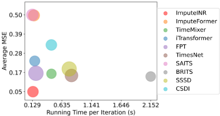
We evaluate the efficiency of the ImputeINR method, with the results presented in Figure 4. On the x-axis, we plot the running time per iteration, while the y-axis represents the average MSE. The size of each bubble is proportional to the number of model parameters.This figure shows that ImputeINR achieves accurate imputation results while requiring relatively little running time. Moreover, the corresponding bubble size suggests that ImputeINR has a relatively small number of model parameters, further emphasizing its efficiency. These results prove that ImputeINR strikes a favorable balance between computational efficiency and imputation accuracy.
5 Conclusion
In this paper, we propose ImputeINR, which achieves effective imputation in extremely sparse scenarios and the imputed data can further enhance the performance of downstream disease diagnosis tasks. In contrast to existing imputation approaches, ImputeINR leverages the sampling frequencyindependent and infinite-sampling frequency capabilities of INR to achieve fine-grained imputation with sparse data.
Acknowledgements
This work was supported by the National Natural Science Foundation of China (Grant Nos. 62202422 and 62372408).
@inproceedings{ijcai2025p1027,
  title     = {ImputeINR: Time Series Imputation via Implicit Neural Representations for Disease Diagnosis with Missing Data},
  author    = {Li, Mengxuan and Liu, Ke and Guo, Jialong and Bu, Jiajun and Wang, Hongwei and Wang, Haishuai},
  booktitle = {Proceedings of the Thirty-Fourth International Joint Conference on
               Artificial Intelligence, {IJCAI-25}},
  publisher = {International Joint Conferences on Artificial Intelligence Organization},
  editor    = {James Kwok},
  pages     = {9241--9249},
  year      = {2025},
  month     = {8},
  note      = {AI4Tech: AI Enabling Technologies},
  doi       = {10.24963/ijcai.2025/1027},
  url       = {https://doi.org/10.24963/ijcai.2025/1027},
}
TY - CPAPER TI - ImputeINR: Time Series Imputation via Implicit Neural Representations for Disease Diagnosis with Missing Data AU - Li, Mengxuan AU - Liu, Ke AU - Guo, Jialong AU - Bu, Jiajun AU - Wang, Hongwei AU - Wang, Haishuai T2 - Proceedings of the Thirty-Fourth International Joint Conference on Artificial Intelligence, IJCAI-25 PB - International Joint Conferences on Artificial Intelligence Organization PY - 2025 SP - 9241 EP - 9249 DO - 10.24963/ijcai.2025/1027 UR - https://doi.org/10.24963/ijcai.2025/1027 ER -Copied
Machine-readable versions of this paper, for tools and AI agents:





