
TCCD: Tree-guided Continuous Causal Discovery via Collaborative MCTS-Parameter Optimization
Proceedings of the Thirty-Fourth International Joint Conference on Artificial Intelligence. AI4Tech: AI Enabling Technologies. Pages 9268-9276.
https://doi.org/10.24963/ijcai.2025/1030
Keywords
- Domain-specific AI4Tech: AI4Telecom
- Advanced AI4Tech: Data-driven AI4Tech
- Advanced AI4Tech: Deep AI4Tech
Abstract
Learning causal relationships in directed acyclic graphs (DAGs) from multi-type event sequences is a challenging task, especially in large-scale telecommunication networks. Existing methods struggle with the exponentially growing search space and lack global exploration. Gradient-based approaches are limited by their reliance on local information and often fail to generalize. To address these issues, we propose TCCD, a framework that combines Monte Carlo Tree Search (MCTS) with continuous gradient optimization. TCCD balances global exploration and local optimization, overcoming the shortcomings of purely gradient-based methods and enhancing generalization. By unifying various causal structure learning approaches, TCCD offers a scalable and efficient solution for causal inference in complex networks. Extensive experiments validate its superior performance on both synthetic and real-world datasets. Code and Appendix are available at https://github.com/jzephyrl/TCCD.
- [Achab et al., 2018] Massil Achab, Emmanuel Bacry, Stéphane Gaïffas, Iacopo Mastromatteo, and Jean- Franc ¸ois Muzy. Uncovering causality from multivariate hawkes integrated cumulants. Journal of Machine Learning Research, 18(192):1-28, 2018.
- [Bhattacharjya et al., 2022] Debarun Bhattacharjya, Karthikeyan Shanmugam, Tian Gao, and Dharmashankar Subramanian. Process independence testing in proxi- mal graphical event models. In Conference on Causal Learning and Reasoning, pages 144-161. PMLR, 2022.
- [Cai et al., 2022] Ruichu Cai, Siyu Wu, Jie Qiao, Zhifeng Hao, Keli Zhang, and Xi Zhang. Thps: Topological hawkes processes for learning causal structure on event sequences. IEEE Transactions on Neural Networks and Learning Systems, 2022.
- [Cheng et al., 2023] Yuxiao Cheng, Runzhao Yang, Tingx- iong Xiao, Zongren Li, Jinli Suo, Kunlun He, and Qiong- hai Dai. Cuts: Neural causal discovery from irregular time-series data. arXiv preprint arXiv:2302.07458, 2023.
- [Chickering, 1996] David Maxwell Chickering. Learning bayesian networks is np-complete. Learning from data: Artificial intelligence and statistics V, pages 121-130, 1996.
- [Chickering, 2002] David Maxwell Chickering. Optimal structure identification with greedy search. Journal of ma- chine learning research, 3(Nov):507-554, 2002.
- [Idé et al., 2021] Tsuyoshi Idé, Georgios Kollias, Dzung Phan, and Naoki Abe. Cardinality-regularized hawkes- granger model. Advances in Neural Information Process- ing Systems, 34:2682-2694, 2021.
- [Itô, 1971] Kiyosi Itô. Poisson point processes attached to markov processes. In Proc. 6th Berk. Symp. Math. Stat. Prob, volume 3, pages 225-240, 1971.
- [Jin et al., 2022] Kebing Jin, Hankz Hankui Zhuo, Zhanhao Xiao, Hai Wan, and Subbarao Kambhampati. Gradient- based mixed planning with symbolic and numeric action parameters. Artif. Intell., 313:103789, 2022.
- [Kocsis and Szepesvári, 2006] Levente Kocsis and Csaba Szepesvári. Bandit based monte-carlo planning. In Eu- ropean conference on machine learning, pages 282-293. Springer, 2006.
- [Lachapelle et al., 2019] Sébastien Lachapelle, Philippe Brouillard, Tristan Deleu, and Simon Lacoste-Julien. Gradient-based neural dag learning. arXiv preprint arXiv:1906.02226, 2019.
- [Li et al., 2022] Wenqian Li, Yinchuan Li, Shengyu Zhu, Yunfeng Shao, Jianye Hao, and Yan Pang. Gflowcausal: Generative flow networks for causal discovery. arXiv preprint arXiv:2210.08185, 2022.
- [Li et al., 2024] Mingjia Li, Shuo Liu, Hong Qian, and Aimin Zhou. A simple yet scalable granger causal struc- tural learning approach for topological event sequences. In The Thirty-eighth Annual Conference on Neural Informa- tion Processing Systems, 2024.
- [Liniger, 2009] Thomas Liniger. Multivariate hawkes pro- cesses. PhD thesis, ETH Zurich, 2009.
- [Liu et al., 2024] Yuequn Liu, Ruichu Cai, Wei Chen, Jie Qiao, Yuguang Yan, Zijian Li, Keli Zhang, and Zhifeng Hao. Tnpar: Topological neural poisson auto-regressive model for learning granger causal structure from event se- quences. In AAAI, pages 20491-20499, 2024.
- [Qiao et al., 2023] Jie Qiao, Ruichu Cai, Siyu Wu, Yu Xiang, Keli Zhang, and Zhifeng Hao. Structural hawkes processes for learning causal structure from discrete-time event se- quences. arXiv preprint arXiv:2305.05986, 2023. IJCAI
- [Runge et al., 2019] Jakob Runge, Peer Nowack, Marlene Kretschmer, Seth Flaxman, and Dino Sejdinovic. Detect- ing and quantifying causal associations in large nonlinear time series datasets. Science advances, 5(11):eaau4996, 2019.
- [Shojaie and Fox, 2022] Ali Shojaie and Emily B Fox. Granger causality: A review and recent advances. An- nual Review of Statistics and Its Application, 9(1):289- 319, 2022.
- [Spirtes and Glymour, 1991] Peter Spirtes and Clark Gly- mour. An algorithm for fast recovery of sparse causal graphs. Social science computer review, 9(1):62-72, 1991.
- [Spirtes et al., 2000] Pater Spirtes, Clark Glymour, Richard Scheines, Stuart Kauffman, Valerio Aimale, and Frank Wimberly. Constructing bayesian network models of gene expression networks from microarray data. 2000.
- [Spirtes et al., 2001] Peter Spirtes, Clark Glymour, and Richard Scheines. Causation, prediction, and search. 2001.
- [Tsamardinos et al., 2006] Ioannis Tsamardinos, Laura E Brown, and Constantin F Aliferis. The max-min hill- climbing bayesian network structure learning algorithm. Machine learning, 65:31-78, 2006.
- [Wang et al., 2021] Xiaoqiang Wang, Yali Du, Shengyu Zhu, Liangjun Ke, Zhitang Chen, Jianye Hao, and Jun Wang. Ordering-based causal discovery with reinforce- ment learning. arXiv preprint arXiv:2105.06631, 2021. IJCAI
- [Xu et al., 2016] Hongteng Xu, Mehrdad Farajtabar, and Hongyuan Zha. Learning granger causality for hawkes processes. In International conference on machine learn- ing, pages 1717-1726. PMLR, 2016.
- [Zhang et al., 2020] Wei Zhang, Thomas Panum, Somesh Jha, Prasad Chalasani, and David Page. Cause: Learning granger causality from event sequences using attribution methods. In International Conference on Machine Learn- ing, pages 11235-11245. PMLR, 2020.
- [Zhang et al., 2021] Keli Zhang, Shengyu Zhu, Marcus Ka- lander, Ignavier Ng, Junjian Ye, Zhitang Chen, and Lujia Pan. gcastle: A python toolbox for causal discovery. arXiv preprint arXiv:2111.15155, 2021.
- [Zheng et al., 2018] Xun Zheng, Bryon Aragam, Pradeep K Ravikumar, and Eric P Xing. Dags with no tears: Con- tinuous optimization for structure learning. In NeurIPS, 2018.
- [Zhou et al., 2013] Ke Zhou, Hongyuan Zha, and Le Song. Learning social infectivity in sparse low-rank networks us- ing multi-dimensional hawkes processes. In Artificial in- telligence and statistics, pages 641-649, 2013.
- [Zhu et al., 2019] Shengyu Zhu, Ignavier Ng, and Zhitang Chen. Causal discovery with reinforcement learning. arXiv preprint arXiv:1906.04477, 2019.
- [Zhuo et al., 2011] Hankz Hankui Zhuo, Qiang Yang, Rong Pan, and Lei Li. Cross-domain action-model acquisition for planning via web search. In ICAPS, 2011.
References were extracted automatically from the PDF and may contain errors.
Full text extracted automatically from the PDF; figures, tables and equations may differ. The PDF is the version of record.
1 Introduction
In various real-world applications, uncovering causal relationships among event types within multi-type event sequences, which are often represented as Directed Acyclic Graphs (DAGs), is a critical and inherently challenging task. In modern telecommunication networks, a single fault can trigger a cascade of alarm events across interconnected devices, driven by complex topological relationships between them. As the scale of networks expands and the complexity of inter-device topologies increases, accurately discerning the causal relationships among these alarm events becomes increasingly challenging [Chickering, 1996; Li et al., 2022].
Recently, Granger causality analysis [Shojaie and Fox, 2022] has become central to causal structure learning. Approaches such as multivariate Hawkes processes [Liniger, 2009] and Poisson point processes [Itˆo, 1971] have been demonstrated to effectively capture event dynamics and intertype interactions. However, traditional causal learning methods [Spirtes and Glymour, 1991; Zhu et al., 2019; Id´e et al., 2021; Bhattacharjya et al., 2022; Qiao et al., 2023] typically assume i.i.d. event sequences, which contradicts the topological dependencies in telecommunication networks. Consequently, the task of effectively learning causal relationships within such complex network topologies has become one of the main challenges in causal learning for alarm-type events.
∗Corresponding author
To overcome the problem of learning Granger causal structures from event sequences under the non-i.i.d. assumption, [Cai et al., 2022] proposed the Topological Hawkes Process (THP), which extends the traditional Hawkes process to time-graph domains for modeling topological event sequences. However, THP struggles with capturing complex generation mechanisms and nonlinear dependencies. Additionally, its reliance on gradient-free optimization and decoupled parameter learning results in inefficient training. To improve modeling capabilities, [Liu et al., 2024] introduced the Topological Neural Poisson Autoregressive model (TNPAR), which utilizes neural point processes to better model event sequences. Despite its enhanced expressiveness, TNPAR suffers from limited training efficiency and scalability due to the lack of analytical likelihood functions. In contrast, S2GCSL [Li et al., 2024] employs a linear kernel to model event activation effects and adopts gradient descent optimization to improve the learning efficiency while maintaining model expressiveness.
Despite advances in causal structure learning, existing methods face critical challenges in large-scale telecommunication networks: (1) The search space for causal structures grows exponentially with network scale and event types, hindering efficient explorations; (2) Dynamic topologies and increasing event types limit the generalization ability of current approaches, making it difficult to accurately estimate spatiotemporal continuous parameters; (3) The lack of effective integration between structure search and parameter optimization makes gradient-based methods fall into local optima, constraining overall model performance.
In response to the above limitations, we present a novel framework, namely TCCD, which integrates Monte Carlo Tree Search (MCTS) with continuous optimization. This combination fully utilizes the exploration-exploitation tradeoff of MCTS to adaptively balance global exploration and local optimization, enabling effective joint optimization of structure search and parameter estimation. Inspired by S2GCSL [Li et al., 2024], we refine the likelihood function design to transform the discrete DAG search problem into a continuous optimization task, thereby enhancing the generalizability of the model. Specifically, this hybrid approach ensures effective exploration of large-scale search spaces while simultaneously improving the accuracy of causal structure inference. Ultimately, our TCCD framework offers a novel solution for large-scale causal structure learning in telecommunications networks, enabling more precise and efficient handling of complex causal relationships.
In summary, we provide the following key contributions:
- We design a tree-guided dynamic parameter learning strategy to achieve joint optimization of structure search and parameter estimation, providing richer search directions for gradient optimization and forming a hierarchical framework of global exploration and local optimization;
- We propose a local optimization mechanism based on influence propagation that enables efficient parameter updates by identifying the impact scope of causal structure changes;
- We develop a hierarchical evaluation approach that unifies different scoring methods, demonstrating strong scalability for large-scale causal inference across multiple event types, complex topologies, and dynamic characteristics.
In light of this, we aim to effectively learn complex causal structures when handling large-scale multi-event data, providing accurate fault prediction and diagnosis support for network operators. Experiments on synthetic and real-world telecommunication fault diagnosis datasets validate the accuracy of the inference results of the TCCD framework in largescale scenarios.
2 RelatedWork
Causal structure learning [Zheng et al., 2018; Tsamardinos et al., 2006; Lachapelle et al., 2019; Wang et al., 2021; Cheng et al., 2023] has emerged as a vital area of research due to its wide-ranging applications. Broadly, existing methods are mainly categorized into constraint-based and scorebased approaches. The PC algorithm [Spirtes et al., 2000] constructs causal graphs through conditional independence tests, while score-based methods search for optimal DAGs using criteria like Bayesian Information Criterion (BIC) or Minimum Description Length (MDL). However, these conventional approaches often struggle with large-scale data. Recent work has focused on multi-type event sequences, particularly through multivariate Hawkes processes based on Granger causality [Shojaie and Fox, 2022; Zhang et al., 2020; Qiao et al., 2023; Xu et al., 2016; Achab et al., 2018]. ADM4 [Zhou et al., 2013] uses kernel methods and L1 regularization for sparse learning, while deep point process methods like RPPN [Zhang et al., 2020] and CAUSE incorporate attention mechanisms and neural networks. To handle non-i.i.d. data, THP [Cai et al., 2022] accounts for topological influences, and TNPAR [Liu et al., 2024] combines topological networks with Granger causality. Recently, S2GCSL [Li et al., 2024] enhanced learning efficiency through linear kernel modeling and gradient descent optimization. Building on these advances, we propose a novel framework TCCD that utilizes tree-guided continuous causal discovery through collaborative optimization of MCTS parameters, with the objective of addressing the challenges of learning causal structures.
3 Preliminaries
In this work, we focus on revealing the causal structure among various event types within sequences of events. Concretely, a multi-type event dataset (or event stream) X = {X(tj)}Mj=1 is a sequence of events, where each event X(tj) = (dj, vj, tj) indicates the occurrence of an event label vj (or synonymously type or variable) at a spatial location dj at a timestamp tj. Here, vj ∈ V denotes the event type, dj ∈ D corresponds to the nodes in the topological graph GD = (D, ED), where ED represents the edges in the graph, and tj ∈ R+ is the event timestamp. The events occur sequentially in the continuous time interval [t1, tT ], with t1 < t2 < · · · < tT . The objective is to explore the causal structure graph (or a directed acyclic graph) GV = (V, EV) among event types, grounded in event sequences X and the topological graph GD. V = {v1, v2, . . . } indicates the set of event types and EV = {e1, e2, . . . } indicates the set of directed edges in the causal graph, where each edge e1 : vi → vj denotes vi causally influences vj.
Definition 1 (State space) S. The state space S represents the set of all possible Directed Acyclic Graphs (DAGs) among event types. When prior causal knowledge Aprior is available, state space S is constructed based on initial state s0 and Aprior. Specifically, causal relationships with vi,j = 1 in Aprior are integrated to generate different DAGs, forming S.
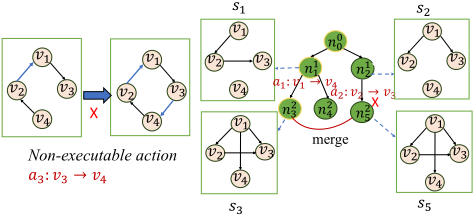
Definition 2 (Action)A. The action set Aconsists of all executable edges that avoid forming cycles. When prior causal knowledge Aprior exists, A is generated based on pairs where vi,j = 0 in Aprior, allowing different edge connections. The action space is defined as A = {av1,v2 : v1 → v2, ..., av4,v3 : v4 → v3}. Each state s has a corresponding set of executable actions A(s) ⊆ A ensuring acyclicity. As shown in Fig. 1, which depicts the causal structures in different states and their corresponding executable actions, blue arrows indicate executable actions, while the red 'X' denotes non-executable actions, such as a3 in state s1 . It is important to note that, since the optimal causal structure cannot be predefined, there is no explicit termination state. Therefore, a termination action Termination(ˆa) is defined, indicating that the termination state has been reached when executed.
Definition 3 (MCTS Tree). The Monte Carlo Tree Search (MCTS) tree consists of nodes and edges that store different types of information. Node nlk : The k-th node at level l in the search tree is defined as a tuple:
where slk represents the current state, A(slk ) is the set of executable actions including Termination(ˆa), N(slk ) tracks visit frequency, and the Hierarchical Potential Score (HPS), denoted as HPS(slk ), quantifies the overall quality of the state. Edge εlk : The edge information for transitions from node nlk is defined as:
where Q(slk , alk vi,vj ) represents the action value for alk vi,vj ∈ A(slk ), and Θlk contains the dynamically optimized causal strength matrix Sw,lk ∈ Rn×n and baseline intensity vector µlk ∈ Rn .
Definition 4 (Intensity function) λ. The event occurrence Otv,d depends on historical event sequences Xh = {(di, vi, ti)|ti < t}, the state s ∈ S, and B0:k. Bk is a set of binary |D| × |D| matrices representing physical connections between devices at geodesic distance k, with Bk di,dj = 1 indicating a connection. The event intensity λv,d t for event type v at device d is given by,
where µv,d is the baseline intensity, Nei(d) represents the set of neighbors for device d, Act(t) is the set of active event types at time t, and αvj,v is the impact of event type vj on event v. ϕ(t - tj)vj,v = e-β(t-tj) is a time-decaying function that models the influence of event vj on v at time t. For simplicity, Nei(d) is abbreviated as N(d), and Act(t) will be denoted as A(t), and we define AN(d, t) = Nei(d) ∩ Act(t) to represent the active neighbors of d at time t.
4 Our TCCD Approach
In this section, we describe how the TCCD framework integrates MCTS with continuous parameter optimization to jointly optimize the causal structure and parameters. In addition, a detailed algorithmic procedure is provided in Appendix A.
4.1 Overview of Our TCCD Approach
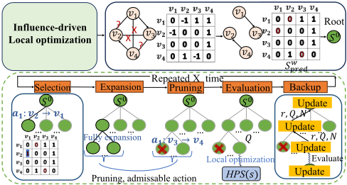
Traditional causal structure learning methods typically treat structure search and parameter optimization as separate tasks. In contrast, we propose the TCCD framework, which innovatively combines Monte Carlo Tree Search (MCTS) with continuous parameter optimization for collaborative optimization. As shown in Fig. 2, TCCD initializes the root node with influence-driven local optimization and employs a treebased dynamic parameter learning strategy, where parameter estimation guides structure exploration, and structural updates trigger efficient local parameter adjustments. Additionally, TCCD introduces a Hierarchical Potential Score function that combines BIC scores, likelihood values, and global consistency to effectively guide the MCTS search and iterative causal structure optimization.
4.2 Influence-Driven Local Optimization
To efficiently process large-scale telecommunication data, we propose a localized optimization mechanism based on influence propagation. The optimization process consists of two main components: log-likelihood function and local parameter updates.
Log-Likelihood Function. Inspired by S2GCSL [Li et al., 2024], we further design a log-likelihood function that integrates current event occurrences X(t0), historical sequences Xh = {(di, vi, ti)|ti < t}, and topological structure B0:k to derive the weighted Granger causal matrix Sw vi,vj = αvi,vj × svi,vj captures the causal influence of event type vi on vj through the Granger causality statistic αvi,vj . Combined with the baseline intensity matrix µ, these parameters form the set Θ = {Sw , µ}, which we optimize using event sequences X = {(di, vi, ti)|i ∈ 1, . . . ,m} through the following likelihood function,
(4)
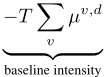
Here, the log-likelihood represents the occurrence probability of the current event at time ti, considering both the baseline intensity µvi,d and the weighted influence from neighboring events (tj < ti and still active) through the exponential decay function ϕ(t) = e-βt . The baseline intensity term reflects the intrinsic occurrence rate of event type v over [0, T], independent of external influences. The compensation integral term corrects for potential future event impacts by integrating the decay effects and causal dynamics of neighbors N(n) and active events A(ti). In addition, the steps to deduce the integral term in the log-likelihood function are as follows,
The final optimization problem follows the S2GCSL[Li et al., 2024] and is defined as,
where λ1 and λ2 are regularization hyperparameters, ||A′ ||1 is the l1-norm of A′ , promoting sparsity in the causal matrix to reduce unnecessary connections and improve interpretability, and h(A′ ) ensures that the deduced causal graph is a directed acyclic graph (DAG) [Zheng et al., 2018].
Local Parameter Updates. To effectively combine continuous optimization with search and improve search efficiency, we propose a novel localized optimization mechanism that dynamically updates parameters only for regions affected by each action. For each action a(vi,vj), we identify the set of affected nodes Naffected = {vi, vj} ∪ {vk | (vi, vk) ∈ EV or (vk, vj) ∈ EV } that includes both event-type nodes vi, vj and their immediate neighbors.
Based on this, we then construct adaptive parameter masks MS ∈ {0, 1}|V|×|V| and Mµ ∈ {0, 1}|V|×|D| , setting elements to 1 for affected nodes (rows and columns in MS and corresponding elements in Mµ) and 0 otherwise. The optimization process employs masked gradient updates with local parameters by Slocal = Sopt ⊙MS and µlocal = µopt ⊙Mµ, where ⊙ denotes the Hadamard product. During backpropagation, gradients are constrained to affected nodes through ∇Sopt = ∇Sopt ⊙ MS and ∇µopt = ∇µopt ⊙ Mµ. Local optimization is performed using Eq.4, tracking the parameter configuration that results in minimal loss. Finally, after the optimization has been completed, only the optimal parameters for the affected nodes are updated to the MCTS nodes. This localized approach significantly reduces computational complexity while maintaining optimization quality by focusing only on relevant parameter subspaces.
4.3 Tree-Guided Continuous-Optimization Casual Discovery
The Monte Carlo Tree Search (MCTS) aims to uncover causal graph structures from observational data by introducing a tree-guided dynamic parameter learning strategy that integrates search and optimization. In the search tree, each node nlk maintains the visit count N(slk ), tracking the frequency of visits to state slk , and the hierarchical potential score HPS(slk ), which evaluates the overall score of slk . For each edge (slk , alk ), assuming a transition from slk to s(l+1)k along (slk , alk ), the action value is defined as Q(slk , alk ) = HPS(s(l+1)k′ ) - HPS(slk ). The Q-function Q(slk , alk ) and parameters Θlk = (Sw,lk , µlk ) are recorded, where the causal strength matrix Sw,lk ∈ Rn×n and baseline intensity vector µlk ∈ Rn are dynamically optimized as the tree expands. Furthermore, in each layer of child nodes, we incorporate the action termination identifier Termination(ˆa) to ensure the optimal node is found.
The search process begins at the root state s0 , progressively selecting and expanding nodes by optimizing the combination of the value function and the exploration reward u(s). Upon reaching a leaf node n′ , all possible child nodes are expanded based on the executable action set A(s′ ), where each child node is evaluated by its hierarchical potential score HPS(schild). These child nodes are then ranked and pruned using a pruning mechanism, after which the updated Q-values and node visit counts N(s) are propagated upwards. Rather than starting with an empty root node, the search space is optimized using an influence-driven local optimization method. Specifically, by utilizing the initialized root node parameters Θinit = (Sw init , µinit), the weight matrix Sw pred = softplus(Sw ) is derived through global optimization, as prescribed by Eq.4, since the root node state is an empty graph with no masks or influence nodes. The action space is constrained by iteratively removing edges with the smallest weights, where the edges to remove are determined by,
After this transformation, the resulting binarized matrix is updated to the root node n0 as the initial state s0 for the subsequent tree search. This transformation reduces the search space by constraining the action set A(s0 ) starting from s0. Subsequently, tree-guided continuous optimization is employed to further guide causal discovery, instead of relying solely on the results of continuous optimization. The entire search process consists of five steps, as illustrated in Fig.2.
Selection. Starting from the root node, we employ the Upper Confidence thresholds (UCB) algorithm [Kocsis and Szepesv´ari, 2006] to select an unexplored node, striking a balance between exploitation and exploration. At each step, an action a is selected to move to a child node, continuing until an unexplored node is found. The selected action a∗ is determined by:
where s′ is the state after action a∗ from state s, Q(s, a) denotes the value of action a, and C controls the explorationexploitation trade-off.
Expansion. For non-terminal leaf nodes, valid actions are generated as:
| Wireless-18 | Micro-25 | |||||||||||
|---|---|---|---|---|---|---|---|---|---|---|---|---|
| Methods | Precision | Recall | F1 | SHD | Precision | Micro-24 Recall | F1 | SHD | Precision | Recall | F1 | SHD |
| PC | 0.5128 | 0.2899 | 0.3704 | - | 0.2553 | 0.1752 | 0.2078 | 155 | 0.2921 | 0.1757 | 0.2194 | 150 |
| GES | 0.5000 | 0.2464 | 0.3301 | 62 | 0.2605 | 0.2263 | 0.2422 | 160 | 0.2078 | 0.2162 | 0.2119 | 179 |
| ADM4 | 0.3727 | 0.5942 | 0.4581 | 49 | 0.2671 | 0.8832 | 0.4102 | 135 | 0.2833 | 0.9189 | 0.4331 | 134 |
| PCMCI | 0.3402 | 0.4783 | 0.3976 | 60 | 0.3333 | 0.4307 | 0.3758 | 126 | 0.2477 | 0.3581 | 0.2928 | 168 |
| Corl | 0.5000 | 0.5362 | 0.6167 | 69 | 0.2778 | 0.0365 | 0.0645 | 135 | 0.2632 | 0.0338 | 0.0599 | 147 |
| THP | 0.7255 | 0.5362 | 0.6167 | 37 | 0.4632 | 0.3212 | 0.3793 | 128 | 0.4118 | 0.2365 | 0.3004 | 140 |
| S2GCSL | 0.6364 | 0.5072 | 0.5645 | 46 | 0.2540 | 0.6934 | 0.3718 | 155 | 0.4786 | 0.3784 | 0.4226 | 124 |
| TCCD | 0.7288 | 0.6232 | 0.6719 | 34 | 0.5470 | 0.4672 | 0.5039 | 115 | 0.4846 | 0.4257 | 0.4532 | 132 |
where IsValid checks action feasibility. Non-root nodes consider a subset of initial state actions to reduce search space. Each node generates a termination-action, Termination(ˆa), inheriting parent parameters and marked terminal. The selected node s∗ is expanded with child nodes n initialized with Q(s, a) = 0.
Evaluation. Each new node state s′ = s ∪ a(vi,vj) inherits and local optimizes its parameters Θ of parent to obtain Θ′ . The potential score of node is measured by the Hierarchical Potential Score (HPS) function:
where α1, α2 and α3 are weights that balance the contributions of BIC, local likelihood and global likelihood in the score function. Llocal(s′ ) and Lglobal(s′ ) are derived from Eq.4, substituting Sw with Sw · s′ , and BIC(s′ ) as in THP [Cai et al., 2022]. Following this, the immediate reward is r(s′ ) = HPS(s′ ) -HPS(s). Hierarchical normalization standardizes child node rewards for comparability, setting identical rewards to zero to indicate no advantage. For terminal states, the potential score of the parent state is used, and visit statistics are initialized for future decisions.
Pruning. After evaluation, a pruning step is conducted to discard child nodes with lower potential scores. Specifically, a threshold θ is determined as θ = sorted(HPS(s), reverse=True)[⌊kthreshold × |HPS(s)|⌋], where kthreshold represents the proportion of child nodes to retain. This process ensures that only the most promising child nodes, likely to yield high returns, are preserved, thereby further reducing the search space.
Backup. During backpropagation, the visit counts N(·) and Q-values for all nodes along the path from the leaf to the root are updated iteratively. The updates propagate bottomup, ensuring that the parent nodes integrate the contributions from their children. The immediate reward of child node r(s′ ) is calculated as HPS(s′ ) - HPS(s), where it denotes the difference between the HPS of a child node and its parent node. The update rules are as follows: For terminal nodes, the Q-value is set directly to the current reward:
For non-terminal nodes, the Q-value is updated iteratively based on a weighted incremental formula:
where s represents a node on the path, and after performing action ˆa, its successor s′ (also on the path) becomes the child node; d represents the depth of the node in the tree, γ is the discount factor controlling the influence of rewards from deeper nodes, and N(s) ← N(s) + 1 denotes the visit count of node s. The update process begins at the leaf node and proceeds sequentially along the path up to the root using a breadth-first traversal method. At each step, the cumulative reward is adjusted using the discount factor γ, ensuring that rewards closer to the leaf node contribute more significantly. Furthermore, node expansion is prohibited after the execution of Termination(ˆa).
5 Experiments
5.1 Experimental Setup
Evaluation Metrics. We evaluated the performance of our TCCD approach with comparison to baselines using realworld metropolitan cellular network alarm data and synthetic datasets. Similar to [Cai et al., 2022; Li et al., 2024], we test the following metrics: Precision, Recall, F1 Score, and Structural Hamming Distance (SHD). Precision measures the proportion of predicted edges that are true among the total predicted edges. Recall quantifies the fraction of actual edges that have been correctly predicted. F1 Score represents the harmonic mean of Precision and Recall, calculated as F1 = 2×Precision×Recall Precision+Recall . SHD denotes the number of edge insertions, deletions, or flips needed to transform a graph into another graph. Also, the detailed implementation and hyperparameters of our experiments are provided in Appendix B.1.
Real-World Metropolitan Cellular Network Alarm Data. We evaluate TCCD on three challenging datasets derived from real-world metropolitan cellular networks, showcased in the PCIC 2021 competition 1 . The first dataset, 18V 55N Wireless (Wireless-18), consists of 18 alarm types, 55 topological network elements, and a total of 34,839
1 https://competition.huaweicloud.com/information/ 1000041487/dataset
alarm events. The other two datasets, 24V 439N Microwave (Micro-24) and 25V 474N Microwave (Micro-25), contain 24 and 25 alarm types, 439 and 474 topological network elements, and 64,599 and 48,573 alarm events, respectively. Remarkably, the Wireless-18 lacks an underlying topological network structure, which demonstrates the applicability of our model. Causal discovery on such datasets aims to uncover causal relationships among alarm types, further validating the effectiveness and generalization capability of our method. Detailed statistics of the datasets are shown in Appendix B.2.
Synthetic Datasets. In addtion, we generate a range of synthetic datasets via the gcatle [Zhang et al., 2021] API, which simulates event sequences using topological Hawkes process [Cai et al., 2022]. The details of the synthetic data generation process and the parameter configurations are provided in Appendix B.3.
Baselines. In experiments, we selected the following causal discovery methods as baselines for comparison: GES [Chickering, 2002], ADM4 [Zhou et al., 2013], PC [Spirtes et al., 2001], PCMCI [Runge et al., 2019], Corl [Wang et al., 2021], THP [Cai et al., 2022] and S2GCSL [Li et al., 2024]. For fairness, we used the optimal parameters as specified in their respective papers (Appendix C). We ran all experiments on a platform with Ubuntu 16.04 on 256GB of memory and an NVIDIA GeForce GTX 1080 Ti GPU.
5.2 Experimental Results
Results on Real-World datasets. Based on the experimental results in Table 1, TCCD consistently outperforms baselines across three real-world datasets. Methods utilizing topological network structures (THP, S2GCSL, and TCCD)
| Datasets | Methods | Pre | Recall | F1 | SHD |
|---|---|---|---|---|---|
| Wireless-18 | TCCD-MCTS TCCD | 0.7273 0.7288 | 0.5797 | 0.6452 | 37 |
| 0.6232 | 0.6719 | 34 | |||
| Micro-24 | TCCD-MCTS | 0.5556 | 0.4380 | 0.4898 | 115 115 |
| TCCD | 0.5470 | 0.4672 | 0.5039 | ||
| Micro-25 | TCCD-MCTS | 0.4841 | 0.4122 | 0.4453 | 132 |
| TCCD | 0.4846 | 0.4257 | 0.4532 | 132 |
achieve higher F1 scores than traditional point process-based approaches (PC, GES, PCMCI), highlighting the importance of spatiotemporal modeling. TCCD outperforms all baselines with the highest F1 score, demonstrating a strong balance between Precision and Recall. On the Wireless-18 dataset, it achieves an F1 of 0.6719, with high Precision 0.7288, Recall 0.6232, and the lowest SHD 34, ensuring accurate causal graph reconstruction. For Micro-24, TCCD maintains optimal performance with the highest F1 0.5039 and Precision 0.5470, alongside the lowest SHD 115, despite higher Recall 0.6934 of S2GCSL. In networks with 25 event types, TCCD
leads with an F1 of 0.4516 and Precision of 0.4809, though SHD is slightly higher than S2GCSL (132 vs. 124). Traditional methods (PC, GES) perform poorly (F1 < 0.37), and ADM4 show high Recall but low Precision, indicating oversensitivity to weak causal signals. In general, TCCD effectively balances inference accuracy and structural correctness, establishing itself as a robust solution for large-scale causal discovery in telecommunication networks.
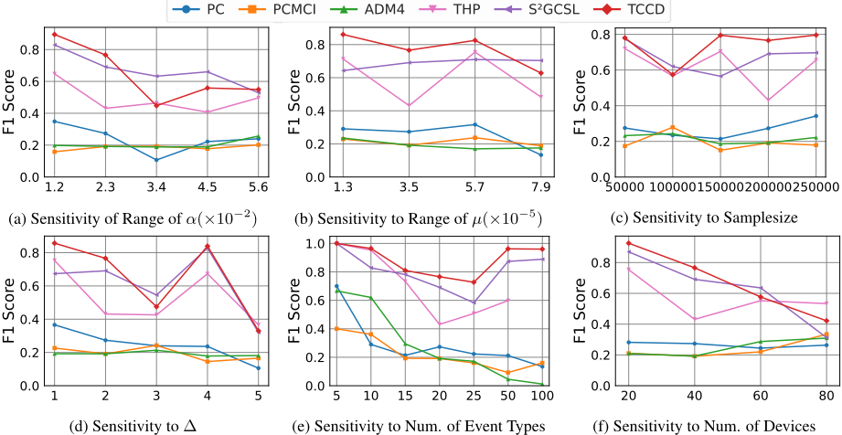
Results on Synthetic Datasets. We further evaluate the performance of TCCD and five baseline models across six dimensions on the synthetic datasets (Fig.3). Fig.3 shows the F1 scores of different methods under various parameter settings (α, µ, δ), with additional evaluation metrics provided in Appendix E. Overall, our TCCD performs well in most cases, achieving relatively high F1 scores across multiple parameter configurations. In particular, it demonstrates strong stability and generalization ability when the sample size is large or the number of event types increases. Although THP [Cai et al., 2022] and S2GCSL [Li et al., 2024] achieve slightly higher F1 scores under certain specific parameter settings, their overall performance is less stable compared to TCCD. Notably, our method maintains superior generalization ability and causal structure learning performance, especially in high-dimensional and complex event sequences.
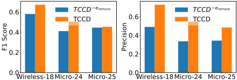
Ablation Study. To validate the effectiveness of the proposed TCCD framework, we conduct ablation experiments on three real-world datasets. Table 2 presents the comparison experimental results between TCCD and its variant TCCD-MCTS , where TCCD-MCTS denotes a simplified version of TCCD that only uses influence-driven local optimization to obtain the initial causal structure s0 without the MCTS-based structure refinement. Additionally, Fig.4 shows the comparison results for another variant TCCD-eremove , which removes the mechanism of eliminating invalid edges from TCCD to assess the impact of this mechanism. As shown in Table 2, one the Wireless-18 dataset, TCCD outperforms TCCD-MCTS in Precision, Recall, and F1, with Recall increasing by 4.35% and F1 by 2.67%. On the more challenging Micro-24 and Micro-25 datasets , while overall performance decreases, TCCD consistently surpasses TCCD-MCTS in Recall and F1. In Micro-24, Recall improves by 2.92% and F1 by 2.41%, despite a slight drop in Precision, indicating better causal recovery. InMicro25, Precision slightly increases, with Recall and F1 improving by 3.29% and 1.78%, respectively. Moreover, the identical SHD values for TCCD and TCCD-MCTS suggest that MCTS enhances structural weights rather than altering causal edge count. Even TCCD-MCTS outperforms the baseline S2GCSL (Table 1), validating the effectiveness of our approach. The superior performance of TCCD can be attributed to two key factors: First, unlike S2GCSL, which primarily rely on statistical correlations, our approach integrates network topology and temporal decay to capture spatiotemporal causality; Second, MCTS enables a more thorough exploration of causal structures, avoiding local optima and improving inference accuracy. Additionally, as shown in Fig.4, removing invalid edges in TCCD-eremove significantly boosts F1 on Wireless-18, highlighting its role in mitigating erroneous causal links. On Micro-24 and Micro-25, TCCD-eremove remains competitive, further confirming the contributions of each module in TCCD.
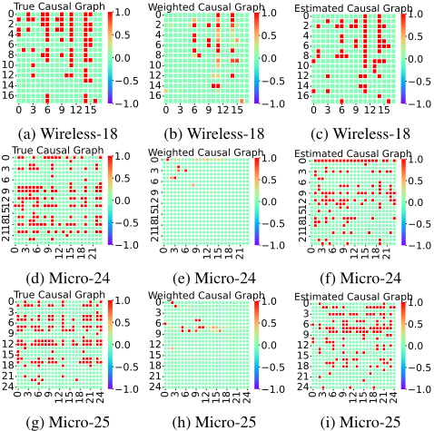
Case Study. Going deeper into the analysis, we evaluate TCCD on three real-world causal networks with N = {18, 24, 25} using True Causal Graph, Weighted Causal Graph (Sw ), and Estimated Causal Graph. Fig.5(a)(b)(c) show how the method identifies local structures in the 18event network by capturing causal relationships 1 → 3, 16 → 14, and 17 → 6 with high fidelity through locality-aware optimization based on influence propagation. For the Micro-24, Fig.5(d)(e)(f) demonstrate effective identification of dense regions (e.g., 8-13) while balancing detailed structural recovery with global sparsity via MCTS. Fig.5(g)(h)(i) reveal the robustness of the method in handling 25 event types. In particular, Fig.5(i) more accurately captures the key causal relationships around nodes 4-12 while reducing false positives in the sparse regions around nodes 20-24. Ultimately, the TCCD framework integrates MCTS with continuous optimization to build accurate causal structures with precision across diverse network scales.
6 Final Remarks
In this paper, we propose TCCD, a framework that combines MCTS with continuous optimization for efficient causal structure learning in large-scale telecommunication networks. By utilizing MCTS's exploration-exploitation strategy and gradient-based optimization, TCCD balances global search and local refinement. It extends the S2GCSL likelihood by integrating discrete DAG search with continuous learning, enabling dynamic feedback to enhance generalization. Future work includes scaling MCTS to larger search spaces via logical action representations [Zhuo et al., 2011; Jin et al., 2022], and adapting the framework to diverse event patterns and temporal dynamics.
Acknowledgments
This work was supported by the National Natural Science Foundation of China (Grant No. 62076263).
@inproceedings{ijcai2025p1030,
  title     = {TCCD: Tree-guided Continuous Causal Discovery via Collaborative MCTS-Parameter Optimization},
  author    = {Liu, Jingjin and Xiao, Yingkai and Zhuo, Hankz Hankui and Wen, Wushao},
  booktitle = {Proceedings of the Thirty-Fourth International Joint Conference on
               Artificial Intelligence, {IJCAI-25}},
  publisher = {International Joint Conferences on Artificial Intelligence Organization},
  editor    = {James Kwok},
  pages     = {9268--9276},
  year      = {2025},
  month     = {8},
  note      = {AI4Tech: AI Enabling Technologies},
  doi       = {10.24963/ijcai.2025/1030},
  url       = {https://doi.org/10.24963/ijcai.2025/1030},
}
TY - CPAPER TI - TCCD: Tree-guided Continuous Causal Discovery via Collaborative MCTS-Parameter Optimization AU - Liu, Jingjin AU - Xiao, Yingkai AU - Zhuo, Hankz Hankui AU - Wen, Wushao T2 - Proceedings of the Thirty-Fourth International Joint Conference on Artificial Intelligence, IJCAI-25 PB - International Joint Conferences on Artificial Intelligence Organization PY - 2025 SP - 9268 EP - 9276 DO - 10.24963/ijcai.2025/1030 UR - https://doi.org/10.24963/ijcai.2025/1030 ER -Copied
Machine-readable versions of this paper, for tools and AI agents:





