
Learning Dynamical Coupled Operator For High-dimensional Black-box Partial Differential Equations
Proceedings of the Thirty-Fourth International Joint Conference on Artificial Intelligence. AI4Tech: AI Enabling Technologies. Pages 9393-9401.
https://doi.org/10.24963/ijcai.2025/1044
Keywords
- Domain-specific AI4Tech: Other AI4Tech applications
- Advanced AI4Tech: Data-driven AI4Tech
Abstract
The deep operator networks (DON), a class of neural operators that learn mappings between function spaces, have recently emerged as surrogate models for parametric partial differential equations (PDEs). However, their full potential for accurately approximating general black-box PDEs remains underexplored due to challenges in training stability and performance, primarily arising from difficulties in learning mappings between low-dimensional inputs and high-dimensional outputs. Furthermore, inadequate encoding of input functions and query positions limits the generalization ability of DONs. To address these challenges, we propose the Dynamical Coupled Operator (DCO), which incorporates temporal dynamics to learn coupled functions, reducing information loss and improving training robustness. Additionally, we introduce an adaptive spectral input function encoder based on empirical mode decomposition to enhance input function representation, as well as a hybrid location encoder to improve query location encoding. We provide theoretical guarantees on the universal expressiveness of DCO, ensuring its applicability to a wide range of PDE problems. Extensive experiments on real-world, high-dimensional PDE datasets demonstrate that DCO significantly outperforms DONs.
- [Adcock et al., 2024] Ben Adcock, Nick Dexter, and Se- bastian Moraga. Optimal deep learning of holomor- phic operators between banach spaces. arXiv preprint arXiv:2406.13928, 2024.
- [Bahdanau, 2014] Dzmitry Bahdanau. Neural machine translation by jointly learning to align and translate. arXiv preprint arXiv:1409.0473, 2014.
- [Bruna and Mallat, 2013] Joan Bruna and S. Mallat. In- variant scattering convolution networks. IEEE Transac- tions on Pattern Analysis and Machine Intelligence, page 1872-1886, Aug 2013.
- [Cao, 2021] Shuhao Cao. Choose a transformer: Fourier or galerkin. Neural Information Processing Systems,Neural Information Processing Systems, Dec 2021.
- [Chen and Chen, 1995] Tianping Chen and Hong Chen. Uni- versal approximation to nonlinear operators by neural net- works with arbitrary activation functions and its applica- tion to dynamical systems. IEEE Transactions on Neural Networks, page 911-917, Jul 1995.
- [Chen et al., 2018] RickyT.Q. Chen, Yulia Rubanova, Jesse Bettencourt, and David Duvenaud. Neural ordinary dif- ferential equations. arXiv: Learning,arXiv: Learning, Jun 2018.
- [Cybenko, 1989] G. Cybenko. Approximation by superpo- sitions of a sigmoidal function. Mathematics of Control, Signals, and Systems, page 303-314, Dec 1989.
- [He et al., 2016] Kaiming He, Xiangyu Zhang, Shaoqing Ren, and Jian Sun. Deep residual learning for image recog- nition. In 2016 IEEE Conference on Computer Vision and Pattern Recognition (CVPR), Jun 2016.
- [Hornik et al., 1989] Kurt Hornik, Maxwell Stinchcombe, and Halbert White. Multilayer feedforward networks are universal approximators. Neural Networks, page 359-366, Jan 1989.
- [Huang et al., 2022] Shudong Huang, Wentao Feng, Chen- wei Tang, and Jiancheng Lv. Partial differential equa- tions meet deep neural networks: A survey. arXiv preprint arXiv:2211.05567, 2022.
- [Jin et al., 2022] Pengzhan Jin, Shuai Meng, and Lu Lu. Mionet: Learning multiple-input operators via ten- sor product. SIAM Journal on Scientific Computing, 44(6):A3490-A3514, 2022.
- [Kissas et al., 2022] Georgios Kissas, Jacob H Seidman, Leonardo Ferreira Guilhoto, Victor M Preciado, George J Pappas, and Paris Perdikaris. Learning operators with cou- pled attention. Journal of Machine Learning Research, 23(215):1-63, 2022.
- [Kovachki et al., 2021] NikolaB. Kovachki, Zongyi Li, Burigede Liu, Kamyar Azizzadenesheli, Kaushik Bhat- tacharya, AndrewM. Stuart, and Anima Anandkumar. Neural operator: Learning maps between function spaces. Cornell University -arXiv,Cornell University -arXiv, Aug 2021.
- [Lee and Oh, 2024] Seungjun Lee and Taeil Oh. Inducing point operator transformer: A flexible and scalable archi- tecture for solving pdes. In Proceedings of the AAAI Con- ference on Artificial Intelligence, volume 38, pages 153- 161, 2024.
- [Leshno et al., 1992] Moshe Leshno, ValdimirYa. Lin, Allan Pinkus, and Shimon Schocken. Multilayer feedforward networks with a non-polynomial activation function can approximate any function. Social Science Research Net- work,Social Science Research Network, Mar 1992.
- [Li et al., 2020] Zongyi Li, Nikola Kovachki, Kamyar Az- izzadenesheli, Burigede Liu, Kaushik Bhattacharya, An- drew Stuart, and Anima Anandkumar. Fourier neural op- erator for parametric partial differential equations. arXiv preprint arXiv:2010.08895, 2020.
- [Li et al., 2022a] Zijie Li, Kazem Meidani, and Amir Barati Farimani. Transformer for partial differential equations' operator learning. Trans. Mach. Learn. Res., 2023, 2022.
- [Li et al., 2022b] Zijie Li, Kazem Meidani, and Amir Barati Farimani. Transformer for partial differential equations' operator learning. arXiv preprint arXiv:2205.13671, 2022.
- [Lu et al., 2019] Lu Lu, Pengzhan Jin, and George Em Kar- niadakis. Deeponet: Learning nonlinear operators for identifying differential equations based on the univer- sal approximation theorem of operators. arXiv preprint arXiv:1910.03193, 2019.
- [Nguyen et al., 2023] Tung Nguyen, Johannes Brandstetter, Ashish Kapoor, Jayesh K Gupta, and Aditya Grover. Cli- max: A foundation model for weather and climate. arXiv preprint arXiv:2301.10343, 2023.
- [Rasp et al., 2020] Stephan Rasp, Peter D Dueben, Sebastian Scher, Jonathan A Weyn, Soukayna Mouatadid, and Nils Thuerey. Weatherbench: A benchmark data set for data- driven weather forecasting. Journal of Advances in Mod- eling Earth Systems, 12(11):e2020MS002203, 2020.
- [Ruthotto and Haber, 2020] Lars Ruthotto and Eldad Haber. Deep neural networks motivated by partial differential equations. Journal of Mathematical Imaging and Vision, 62(3):352-364, 2020.
- [Sriperumbudur et al., 2010] BharathK.
- Sriperumbudur, Kenji Fukumizu, and GertR.G. Lanckriet. Universality, characteristic kernels and rkhs embedding of measures. arXiv: Machine Learning,arXiv: Machine Learning, Mar 2010.
- [Verma et al., 2024] Yogesh Verma, Markus Heinonen, and Vikas Garg. Climode: Climate and weather forecast- ing with physics-informed neural odes. arXiv preprint arXiv:2404.10024, 2024.
References were extracted automatically from the PDF and may contain errors.
Full text extracted automatically from the PDF; figures, tables and equations may differ. The PDF is the version of record.
1 Introduction
Solving black-box parametric partial differential equations (PDEs) remains a significant challenge in many scientific and engineering disciplines [Zachmanoglou and Thoe, 1986]. Traditional methods, such as the finite element method, are computationally expensive and poorly scalable for large-scale or real-time problems. This is particularly problematic in scenarios where large amounts of data need to be processed quickly, such as uncertainty quantification, optimization under uncertainty, or optimal experimental design.
The emergence of neural networks has provided a powerful alternative for approximating solutions to complex problems. Some studies directly apply neural networks [Ruthotto and Haber, 2020; Huang et al., 2022], while others use Neural ODEs [Chen et al., 2018; Verma et al., 2024] to learn mappings between infinite-dimensional function spaces. However, both approaches face distinct challenges: neural networks often struggle with issues such as fixed query locations, whereas Neural ODEs require numerical integration, which can lead to significant error accumulation over time.
Therefore, the Deep Operator Network (DeepONet) [Lu et al., 2019] has gained prominence, offering a more specialized framework for learning mappings between function spaces. DeepONets represent a mapping F(u) from a function u to an output function at a query location y as:
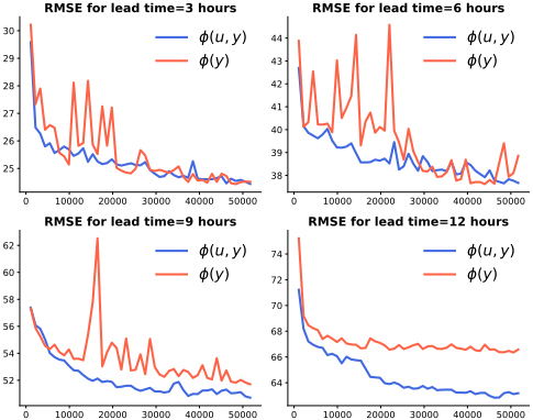
where ϕi(y) are functions mapping the query location y to a finite-dimensional vector, and vi(u) are functionals mapping the input u to real numbers in R. They form a linear combination to approximate the true operator. DONs confront three fundamental limitations. First, the mapping ϕ from the low-dimensional input y to high-dimensional latent representations (Fig. 1) induces inevitable information bottlenecks, compromising approximation learning and inducing training instability. Second, existing approaches exhibit deficiencies in encoding mechanisms for input functions and query locations, constraining their capacity for approximation. Third, while the original DeepONet architectures have universal approximation guarantees, many derivative formulations sacrifice this theoretical foundation without rigorous justification, undermining their reliability in scientific computing applications.
For instance, MIONet [Jin et al., 2022] enhances the expressivity of the operator v by incorporating multi-input function information. However, it still fails to address training stability issues effectively. The LOCA method [Kissas et al., 2022] enables efficient approximation of the operator ϕ by calculating kernels between input and query locations. It struggles with early training stability and has shown limited practical effectiveness. On the other hand, IPOT [Lee and Oh, 2024] introduces lightweight operators based on attention mechanisms, aiming to improve efficiency. However, these approaches still do not guarantee the desired approximation properties. Additionally, related neural operator architectures and their variants, such as those in [Li et al., 2020; Li et al., 2022a], further highlight the challenges in achieving both stability and approximation guarantees.
To address these challenges, we propose the Dynamical Coupled Operator (DCO), a novel operator in the DeepONet class. We introduce a new approximation formulation for ϕ that incorporates temporal dynamics to learn an inputquery coupled function. By leveraging function information, we tackle the issue of mapping low-dimensional inputs to high-dimensional information bottlenecks and improve robustness. Additionally, we introduce an adaptive spectral input function encoder based on empirical mode decomposition to decompose non-stationary functions, thereby enhancing function representation. Furthermore, we propose a hybrid location encoding mechanism to improve query location encoding.
Overall, our method is compared with other operator method in Tab 1 and contributions are as follows:
- Dynamically Coupled Representations: We integrate temporal dynamics to learn an input-query coupled function, address the information bottleneck and and improve robustness.
- Adaptive spectral Input Function Encoder and Hybrid Location Encoding: We integrate EMD to handle non-stationary functions and utilize hybrid location encoding techniques to enhance model performance.
- Theoretical Guarantees of Universality: We prove that the proposed framework satisfies the universal approximation property, meaning it can approximate any continuous operator with arbitrary accuracy.
- Numerical Experiments: We conduct extensive numerical experiments on real-world physical systems, demonstrating that DCO outperforms models in the DON class.
| Class | Method | Universality Guarantee | Dynamics- informed | Information bot- tlenecks inMap- ping |
|---|---|---|---|---|
| Non-DON Class | OFormer IPOT | ✗ ✗ | ✗ ✗ | ✓ ✓ |
| DON Class | DeepONet FNO LOCA DCO (ours) | ✓ ✓ ✓ ✓ | ✗ ✗ ✗ ✓ | ✗ ✗ ✗ ✓ |
2 RelatedWork
2.1 Operator Learning
Neural operators, which approximate mappings between input and output function spaces, include DeepONet [Lu et al., 2019], which utilizes branch and trunk networks to handle inputs and query positions, demonstrating strong approximation capabilities. The Fourier Neural Operator (FNO) [Li et al., 2020] operates in the frequency domain to capture global dependencies but lacks the ability to generalize to arbitrary query locations. Extensions like MIONet [Jin et al., 2022] improve flexibility of multiple input functions. LOCA [Kissas et al., 2022] calculates kernels between input function locations and query locations, enabling efficient approximation of query location representations. Some attentionbased frameworks, including Galerkin Transformers [Cao, 2021] and OFormer [Li et al., 2022b], employ cross-attention mechanisms to enhance adaptability to diverse input conditions. These models reduce computational costs while maintaining flexibility. IPOT [Lee and Oh, 2024] offers flexibility in processing arbitrary discretization. However, DONs do not leverage dynamic information and fail to address information bottlenecks, while non-DONs approaches lack universal approximation guarantees. In contrast, we address these issues by proposing a universal approximation guarantee and a more flexible operator formulation.
2.2 Approximation Theory
The approximation properties of neural networks have been extensively studied, with a focus on network structures such as feedforward neural networks [Cybenko, 1989; Hornik et al., 1989; Leshno et al., 1992] and residual networks [He et al., 2016]. These traditional networks often use a fixed architecture, with weights adjusted to approximate target functions. Recent theoretical advancements have extended universal approximation results to infinite-dimensional function spaces and nonlinear operators. For instance, Chen and Chen [Chen and Chen, 1995] demonstrated that neural networks can approximate nonlinear operators, providing a foundational theoretical basis for operator learning. Building on this, architectures like DeepONet [Lu et al., 2019], LOCA [Kissas et al., 2022], holomorphic operators [Adcock et al., 2024], and neural operators [Kovachki et al., 2021] have emerged, focusing on learning mappings between infinite-dimensional Banach spaces. While these methods primarily rely on static state representations, they lack flexibility in incorporating dynamic information, which limits their robustness and scalability.
3 ProblemFormulation
| Symbol | Description |
|---|---|
| [n] | The set {1, . . . , n} ⊂ N. Element-wise product of u and v. |
| u ⊙ v | |
| C(A,B) | Continuous functions from space A to space B. |
| ∆n | n-dimensional simplex. |
| X | Domain for input functions. |
| Y | Domain for output functions. |
| x | Input function arguments. |
| y | Output function arguments (queries). |
| u | Input function in C(X,Rdu ). |
| s | Output function in C(Y,Rds ). |
| F | Mapping input functions to output functions. |
| ψ(y) | Query encoding function. |
| v(u), k(u) | Feature encoding function. |
| ϕ(u, y) | State query coupled-kernel function. |
In this section, we aim to formalize the operator learning problem, specifically the relationship between input and output functions as defined by the symbols in Table 2.
Given N pairs of dynamic series of input functions and output functions {uℓt-1 (x), uℓt (x), sℓ (y)}Nℓ=1 , where uℓ ∈ C(X,Rdu ) and sℓ ∈ C(C(X,Rdu ) × Y,Rds ), the data pairs are assumed to be generated by an unknown ground truth operator G, defined as:
which maps an input function uℓt-1 (x) to its corresponding output function sℓ (uℓt (x), y).
Our goal is to learn an operator F such that for each function pair, the learned operator should satisfy:
and for ℓ = 1, . . . , N, we want:
We discuss this from the perspective of a simplified version, this formulation can be applied to various scenarios. For instance, consider a case where u represents a temperature field over the Earth's surface, and X is the spatial domain. The output s could be the pressure field sampled at specific locations Y. The operator F would then predict the pressure fields given new temperature distributions.
4 Method
We construct our model in two steps, inspired by attention mechanisms. First, we map the input function ut-1 to a feature vector v(ut-1) ∈ Rn . For each output location y and input function ut, we enhance the model by coupling the current state ut and y using an attention kernel, as in formula 1, to obtain an approximating function ϕ : C(X,Rdu ) × Y → Rn×ds through ψ(y) and k(ut). Here, σ denotes the softmax function. The forward pass of the proposed model is written as follows:
In this section, we will describe how the functions v and ϕ are constructed through ψ and k.
4.1 Adaptive Spectral Input Function Encoder
In our approach, the feature mappings k(·) and v(·) are constructed through two main operations. The first operation is the function E, which maps an input function u to a finite - dimensional vector space Rd :
Traditional spectral methods, such as the Fourier Transform and wavelet scattering networks[Bruna and Mallat, 2013] using in LOCA, offer effective feature representations but struggle with non-linear and non-stationary functions. For instance, Fourier Transform is sensitive to small deformations, while wavelet scattering relies on fixed basis functions that may not adapt to input signals' intrinsic characteristics. To address these challenges, we use Empirical Mode Decomposition (EMD) for feature extraction.
EMD is a data - driven technique that decomposes signals into multiscale oscillatory components, making it well - suited for non - linear and non - stationary signals. EMD decomposes an input signal u into Intrinsic Mode Functions (IMFs), denoted as χi(m), where each IMF captures an oscillatory component of the signal at a particular scale. The decomposition can be expressed as:
where d is the number of IMFs and M is the sequence length. Each IMF χi(m) satisfies: The difference between zero crossings and extrema is at most 1.
The mean of the upper and lower envelopes of χi(m) is zero.
This decomposition allows for the extraction of features at multiple scales. We define the mapping E(·) using the first d IMFs, along with the input signal u:
where ⊕ denotes concatenation.
After obtaining the finite - dimensional representation of u, we apply functions q and f, drawn from universal function approximators (e.g., fully connected neural networks), to obtain the feature representations:
4.2 Hybrid Query Locations Encoding
To encode the query locations y, we design ψ(y) to capture both intrinsic location information and the relative distance to the input function locations. To achieve this, we adopt a hybrid encoding scheme that combines a normalized radial basis function (RBF) kernel with discrete Fourier encoding.
The normalized RBF kernel is defined as:
where κ(y, y′ ) quantifies the similarity between y and y′ ∈ Y. Using a set of reference points {y′i }ni=0 , we compute the RBF - based features as:
where W1 ∈ R(n+1)×d is a learnable weight matrix.
To complement the localized features provided by the RBF kernel, we apply discrete Fourier encoding to capture periodic features of y. The Fourier features are given by:
where {ci}Ni=1 are predefined Fourier frequencies. Finally, the combined features a and b are concatenated and passed through a universal function approximator g to compute the final representation:ψ(y) = g(a ⊕ b) ∈ RD ,
This hybrid encoding effectively captures both localized and periodic characteristics of y, enhancing the expressivity of y representation.
4.3 Input-Query Coupled Function
To construct the state-dependent representation ϕ, we couple the input function ut with the query points y. First, we encode the current state ut using the feature encoder k, and encode the query points y ∈ Y using ψ. Inspired by by attention mechanism[Bahdanau, 2014], we compute a tensor-matrix product between ψ(y) and k(ut), followed by applying the softmax operation σ : Rn → ∆n to the rows. This softmax operation bounds the values of ϕ, where ∆n represents the probability simplex:
This formulation allows the representation ϕ(ut, y) to capture both the current state dependencies through the attention mechanism and spatial correlations via the positional encoding of y. By combining these components, the model is able to learn a richer and more expressive mapping.
4.4 Loss Function
To account for the geometric properties of a sphere, we employ a latitude-weighted mean squared error (MSE) loss function[Nguyen et al., 2023]:
where the latitude weight L(y) = cos(h) 1H ∑Hy′ cos(y′ ) , and h represents the latitude of the grid point y. Ω denotes the set of all grid points, and N is the total number of samples.
5 Theoretical Guarantees of Universality
In this section we give conditions under which the DCO model is universal. There exist multiple definitions of universality present in the literature, for example see[Sriperumbudur et al., 2010]. To be clear, we formally extend the definition we use below.
Definition 1 (Universality). Let X ⊂ Rdx , Y ⊂ Rdy , and U ⊂ C(X,Rdu ) be compact sets. A class of operators A is said to be universal if for any continuous operator
and any ϵ > 0, there exists an operator F ∈ A such that:
To explore the universality properties of our model we note that evaluation of the model can be written as
We will show that our model with the bounded normalization, state-query coupling ϕ and Adaptive spectral input function encoder v are universal by adding these components back one at a time. First, the following theorem shows that bounded normalization, state-query coupling ϕ does not reduce the approximation power of this class of operators.
Theorem 1 (DCO Preserves Universality). Let U ⊂ C(X, Rdu ) be a compact set, and let
be a continuous operator, where X ⊂ Rdx and Y ⊂ Rdy are compact. Then, for every ϵ > 0, there exist n ∈ N, functionals vj : U → R for j ∈ [n], and functions ϕj : C(X , Rdu ) × Y → Rn×ds , such that:
Lastly, we present a result showing that a particular architecture choice for the input feature encoder v also preserves universality. We show that EMD can be used to construct a universal class of functionals on C(X, Rdu ).
Proposition 1 (EMD Encoding Preserves Universality). Let Ad ⊂ C(Rd ,Rn ) be a set of functions dense in C(Rd ,Rn ), and {ei}∞i=1 a set of basis functions such that for some compact set U ⊂ C(X,Rd ). Let Ed : U → Rd denote in 4.1. Then for any continuous mapping h : U → Rn and any ϵ > 0, there exist d and f ∈ Ad such that:
Proof. The proof is provided in Appendix B.
For example, if our compact space of input functions U is contained in C 1 (X,Rdu ), the architecture proposed is expressive enough to approximate any functional from U → R.
| Metric | Model | 3h | 6h | ||||||||||
|---|---|---|---|---|---|---|---|---|---|---|---|---|---|
| t2m | u10 | v10 | t850 | z500 | Avg | t2m | u10 | v10 | t850 | z500 | Avg | ||
| DeepONet | 0.0180 | 0.1642 | 0.1990 | 0.0088 | 0.0022 | 0.0785 | 0.0278 | 0.2173 | 0.3015 | 0.0130 | 0.0045 | 0.1128 | |
| MSE LOCA | 0.0085 | 0.1407 | 0.1631 | 0.0073 | 0.0013 | 0.0642 | 0.0105 | 0.1853 | 0.2457 | 0.0103 | 0.0031 | 0.0910 | |
| IPOT | 0.0071 | 0.1326 | 0.1549 | 0.0071 | 0.0013 | 0.0606 | 0.0088 | 0.1771 | 0.2411 | 0.0100 | 0.0031 | 0.0880 | |
| DCO (ours) | 0.0046 | 0.1298 | 0.1507 | 0.0062 | 0.0011 | 0.0585 | 0.0061 | 0.1755 | 0.2391 | 0.0088 | 0.0026 | 0.0864 | |
| DeepONet | 2.8472 | 2.2346 | 2.1189 | 1.4746 | 163.2574 | 34.3866 | 3.5376 | 2.5708 | 2.6074 | 1.7870 | 232.8443 | 48.6694 | |
| RMSE LOCA | 1.9572 | 2.0683 | 1.9183 | 1.3371 | 127.6338 | 26.9829 | 2.1819 | 2.3734 | 2.3540 | 1.5919 | 193.1909 | 40.3384 | |
| IPOT | 1.7887 | 2.0073 | 1.8692 | 1.3249 | 126.4169 | 26.6814 | 1.9961 | 2.3206 | 2.3316 | 1.5677 | 194.4303 | 40.5293 | |
| DCO (ours) | 1.4393 | 1.9862 | 1.8439 | 1.2319 | 114.1292 | 24.1261 | 1.6630 | 2.3099 | 2.3225 | 1.4699 | 176.5892 | 36.8709 | |
| Model | 9h | 12h | |||||||||||
| t2m | u10 | v10 | t850 | z500 | Avg | t2m | u10 | v10 | t850 | z500 | Avg | ||
| DeepONet | 0.0353 | 0.2784 | 0.4250 | 0.0178 | 0.0072 | 0.1527 | 0.0365 | 0.3405 | 0.5523 | 0.0226 | 0.0111 | 0.1926 | |
| MSE LOCA | 0.0126 | 0.2437 | 0.3471 | 0.0143 | 0.0056 | 0.1247 | 0.0144 | 0.3017 | 0.4489 | 0.0185 | 0.0084 | 0.1584 | |
| IPOT | 0.0102 | 0.2347 | 0.3581 | 0.0139 | 0.0059 | 0.1246 | 0.0123 | 0.2921 | 0.4378 | 0.0179 | 0.0091 | 0.1539 | |
| DCO (ours) | 0.0077 | 0.2331 | 0.3352 | 0.0122 | 0.0048 | 0.1186 | 0.0087 | 0.2913 | 0.4287 | 0.0158 | 0.0075 | 0.1504 | |
| DeepONet | 3.9930 | 2.9093 | 3.0940 | 2.0930 | 294.5810 | 61.3341 | 4.0593 | 3.2168 | 3.5260 | 2.3544 | 366.2193 | 75.8752 | |
| RMSE LOCA | 2.3876 | 2.7218 | 2.7972 | 1.8727 | 260.0438 | 53.9646 | 2.5507 | 3.0280 | 3.1804 | 2.1309 | 318.4295 | 65.8639 | |
| IPOT | 2.1443 | 2.6708 | 2.8402 | 1.8452 | 267.1718 | 55.3345 | 2.3596 | 2.9794 | 3.1402 | 2.0980 | 331.2527 | 68.3660 | |
| DCO (ours) | 1.8669 | 2.6620 | 2.7496 | 1.7298 | 241.0392 | 50.0095 | 1.9815 | 2.9759 | 3.1094 | 1.9686 | 300.7749 | 62.1621 | |
6 Numerical Experiments
Unlike previous operator experiments, which typically involve low - dimensional and relatively simple datasets, we conduct experiments on a real - world, high - dimensional black - box PDE dataset. In this section, we present a comprehensive set of experiments to evaluate the performance of the proposed method. These experiments aim to assess the model's effectiveness in solving high - dimensional black - box partial differential equations. Beyond ablation studies, we focus on addressing the following key research questions 1 :
- How does the model perform in predicting various physical quantities compared to baselines?
- How well does the model train to predict unseen query locations compared to state-of-the-art DONs?
6.1 Experimental Setup
Datasets. We use the preprocessed 3 - hour increment ERA5 dataset from WeatherBench [Rasp et al., 2020], which contains governing black - box PDEs. We consider a dimensionality of du = 54 for input function and ds = 5 for output function from the ERA5 dataset: ground temperature (t2m), atmospheric temperature (t), geopotential (z), and ground wind vector (u10, v10). We use data at three different scales for evaluation. More details can be found in Appendix C.
Metrics. We evaluate our benchmarks using two commonly used metrics: latitude - weighted RMSE and latitude
1 https://github.com/ResearchGroupHdZhang/DCO
- weighted MSE. More metrics details can be found in Appendix D.
Baselines. To evaluate the effectiveness of our proposed method, we compare it with several baseline methods:
- DeepONet[Lu et al., 2019]: A foundational neural operator model that approximates functions using a branch - trunk network architecture, offering a rigorous mathematical framework based on approximation theory.
where g is the function representing query location y, and v is the function representing the input function u.
- LOCA[Kissas et al., 2022]: An extension of DeepONet that integrates the Wavelet Scattering Network and attention mechanisms to enhance the coupling between the input and query coordinates
where κ : Y × Y → R is the kernel, σ is the softmax function, v is the input feature encoder, and g is the proposed score function.
- IPOT[Lee and Oh, 2024]: A neural operator framework designed for optimal transport problems, which employs a differentiable iterative solver to approximate transport maps.
| Metric | Model | 3h | 6h | ||||||||||
|---|---|---|---|---|---|---|---|---|---|---|---|---|---|
| t2m | u10 | v10 | t850 | z500 | Avg | t2m | u10 | v10 | t850 | z500 | Avg | ||
| DeepONet | 0.0161 | 0.1574 | 0.1913 | 0.0084 | 0.0016 | 0.0750 | 0.0257 | 0.2025 | 0.2748 | 0.0119 | 0.0038 | 0.1037 | |
| LOCA | 0.0097 | 0.1477 | 0.1757 | 0.0079 | 0.0013 | 0.0685 | 0.0117 | 0.1901 | 0.2534 | 0.0107 | 0.0031 | 0.0938 | |
| MSE IPOT | 0.0076 | 0.1380 | 0.1672 | 0.0077 | 0.0013 | 0.0643 | 0.0093 | 0.1810 | 0.2485 | 0.0104 | 0.0032 | 0.0905 | |
| DCO (ours) | 0.0049 | 0.1351 | 0.1623 | 0.0065 | 0.0010 | 0.0619 | 0.0063 | 0.1802 | 0.2436 | 0.0091 | 0.0026 | 0.0883 | |
| DeepONet | 2.6937 | 2.1884 | 2.0781 | 1.4357 | 138.5084 | 29.3809 | 3.3961 | 2.4819 | 2.4898 | 1.7126 | 213.0866 | 44.6334 | |
| LOCA | 2.0975 | 2.1196 | 1.9919 | 1.3903 | 125.9023 | 26.7003 | 2.2968 | 2.4049 | 2.3911 | 1.6252 | 194.2024 | 40.5841 | |
| RMSE IPOT | 1.8505 | 2.0490 | 1.9426 | 1.3725 | 124.3201 | 26.307 | 2.0456 | 2.3461 | 2.3677 | 1.5990 | 196.5081 | 40.973 | |
| DCO (ours) | 1.4816 | 2.0269 | 1.9138 | 1.2687 | 112.2921 | 23.797 | 1.6933 | 2.3411 | 2.3447 | 1.4921 | 176.9052 | 36.96 | |
| Metric | Model | 9h | 12h | |||||||||
|---|---|---|---|---|---|---|---|---|---|---|---|---|
| t2m | u10 | v10 | t850 | z500 | Avg t2m | u10 | v10 | t850 | z500 | Avg | ||
| DeepONet | 0.0340 | 0.2613 | 0.3948 | 0.0167 | 0.0064 | 0.1426 0.0369 | 0.3231 | 0.5236 | 0.0217 | 0.0100 | 0.1830 | |
| LOCA | 0.0137 | 0.2480 | 0.3553 | 0.0147 | 0.0057 | 0.1275 0.0157 | 0.3064 | 0.4575 | 0.0189 | 0.0086 | 0.1614 | |
| MSE IPOT | 0.0107 | 0.2384 | 0.3662 | 0.0143 | 0.0061 | 0.1271 0.0129 | 0.2960 | 0.4462 | 0.0184 | 0.0093 | 0.1565 | |
| DCO (ours) | 0.0079 | 0.2370 | 0.3399 | 0.0124 | 0.0049 | 0.1204 0.0089 | 0.2944 | 0.4335 | 0.0160 | 0.0076 | 0.1521 | |
| DeepONet | 3.9053 | 2.8190 | 2.9828 | 2.0250 | 277.4299 | 57.8324 4.0641 | 3.1341 | 3.4335 | 2.3062 | 346.3043 | 71.8484 | |
| LOCA | 2.4893 | 2.7461 | 2.7223 | 2.0955 | 243.8145 | 53.3789 2.6502 | 3.0916 | 3.2645 | 2.1797 | 298.6246 | 63.5578 | |
| RMSE IPOT | 2.1963 | 2.6921 | 2.8724 | 1.8737 | 270.2282 | 55.973 2.4151 | 2.9991 | 3.1704 | 2.1239 | 335.0262 | 69.147 | |
| DCO (ours) | 1.8939 | 2.6847 | 2.7694 | 1.7478 | 241.9643 | 50.21 2.0089 | 2.9920 | 3.1272 | 1.9859 | 301.9195 | 62.41 | |
Implementation Details. To comprehensively evaluate our method, we conducted experiments using different lead times (3, 6, 9, 12 hours) in both the black-box PDE solving and query location generation tasks. All the training details can be found in Appendix E.
6.2 Experiments on Solving Black-box PDEs
To answer first question, We evaluate our model's performance in predicting multiple forward time steps of black-box PDEs. As shown in Table 3, our model significantly outperforms DONs and IPOT in terms of MSE and RMSE across all time steps and physical quantities in small scale PDEs. For instance, at 3h, our model achieves an average MSE of 0.0619, compared to 0.0750 for DeepONet and 0.0643 for IPOT. Similarly, at 6h, our model's MSE is 0.0883, while DONs and IPOT report 0.1037 and 0.0905, respectively. In terms of RMSE, at 3h, our model achieves a value of 23.797, which is a notable improvement over the 29.3809 from DeepONet and 26.307 from IPOT. At 6h, the RMSE of our model (36.96) is also significantly lower than that of DeepONet (44.6334) and IPOT (40.973). These results demonstrate the superior predictive accuracy and generalization ability of our model.
6.3 Experiments on Query Locations Generation
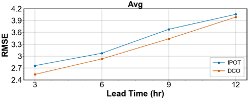
To answer the first question, we evaluate our model's ability to generalize to unseen query locations, specifically predicting from small-scale to medium-scale. As shown in Table 4, our model consistently outperforms baselines in both MSE and RMSE for unseen queries. At 3h, our model achieves an average MSE of 0.0619 and RMSE of 23.797, significantly lower than DeepONet's 0.0750 and 29.3809, and IPOT's 0.0643 and 26.307. Similarly, at 6h, the average MSE and RMSE are 0.0883 and 36.96, compared to DeepONet's 0.1037 and 44.6334, and IPOT's 0.0905 and 40.973. These results demonstrate the superior generalization capability of our model for unseen query points. As shown in Fig. 2, we also conduct zero-shot unseen query generation experiments to further highlight the superior performance of our model, specifically from small-scale predictions to large-scale ones. More details can be found in Appendix F.
6.4 Ablation Study and Visualization
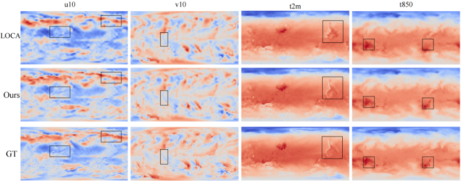
As shown in Table 5, we conducted an ablation study to evaluate the impact of different components on model performance. Removing the Wavelet scattering (w/o B) leads to a decrease in performance across all time intervals, with higher MSE and RMSE values. Similarly, removing the hybrid query location encoding (w/o A) results in a significant drop in performance, especially in the RMSE metric. Our full model, which includes both components A and B, achieves the best performance, demonstrating the importance of both components in optimizing model accuracy and robustness. As shown in Fig 1, and the complete comparison of training stability can be found in Appendix G. In Fig 3, we campare to 4 physical quantities. it can be seen that our method also outperforms in terms of intricate scale, as indicated by the black box.
| Metric | Model | 3h | 6h | ||||||||||
|---|---|---|---|---|---|---|---|---|---|---|---|---|---|
| t2m | u10 | v10 | t850 | z500 | Avg | t2m | u10 | v10 | t850 | z500 | Avg | ||
| MSE | w/o A | 0.0119 | 0.1534 | 0.1869 | 0.0079 | 0.0012 | 0.0723 | 0.0144 | 0.1970 | 0.2685 | 0.0108 | 0.0031 | 0.0987 |
| w/o B | 0.0056 | 0.1364 | 0.1651 | 0.0069 | 0.0011 | 0.0630 | 0.0074 | 0.1785 | 0.2384 | 0.0096 | 0.0028 | 0.0873 | |
| ours | 0.0049 | 0.1351 | 0.1623 | 0.0065 | 0.0010 | 0.0619 | 0.0063 | 0.1802 | 0.2436 | 0.0091 | 0.0026 | 0.0884 | |
| RMSE | w/o A | 2.3244 | 2.1605 | 2.0539 | 1.3942 | 122.8667 | 26.1599 | 2.5545 | 2.4478 | 2.4614 | 1.6273 | 192.0525 | 40.2287 |
| w/o B | 1.5949 | 2.0366 | 1.9306 | 1.3023 | 116.0252 | 24.5779 | 1.8286 | 2.3301 | 2.3190 | 1.5342 | 183.9327 | 38.3889 | |
| ours | 1.4816 | 2.0269 | 1.9138 | 1.2687 | 112.2921 | 23.797 | 1.6933 | 2.3411 | 2.3447 | 1.4921 | 176.9052 | 36.96 | |
| Metric | Model | 9h | 12h | ||||||||||
|---|---|---|---|---|---|---|---|---|---|---|---|---|---|
| t2m | u10 | v10 | t850 | z500 | Avg | t2m | u10 | v10 | t850 | z500 | Avg | ||
| MSE | w/o A | 0.0177 | 0.2528 | 0.3653 | 0.0149 | 0.0058 | 0.1313 | 0.0196 | 0.3117 | 0.4771 | 0.0190 | 0.0092 | 0.1673 |
| w/o B | 0.0090 | 0.2339 | 0.3380 | 0.0133 | 0.0057 | 0.1199 | 0.0103 | 0.2924 | 0.4406 | 0.0176 | 0.0088 | 0.1539 | |
| ours | 0.0079 | 0.2370 | 0.3399 | 0.0124 | 0.0049 | 0.1204 | 0.0089 | 0.2944 | 0.4335 | 0.0160 | 0.0076 | 0.1521 | |
| RMSE | w/o A | 2.8324 | 2.7729 | 2.8700 | 1.9158 | 264.6731 | 55.0129 | 2.9766 | 3.0781 | 3.2790 | 2.1584 | 332.3575 | 68.77 |
| w/o B | 2.0137 | 2.6668 | 2.7607 | 1.8093 | 262.3314 | 54.3164 | 2.1510 | 2.9810 | 3.1511 | 2.0764 | 325.18 | 67.11 | |
| ours | 1.8939 | 2.6847 | 2.7694 | 1.7478 | 241.9643 | 50.21 | 2.0089 | 2.9920 | 3.1272 | 1.9859 | 301.9195 | 62.41 | |
7 Conclusion
In this work, we introduced the Dynamical Coupled Operator (DCO), a novel framework for learning mappings between continuous function spaces. DCO overcomes key limitations of traditional neural operators by incorporating temporal dynamics and coupling input representations with query locations. This design reduces information loss, enhances the model's ability to capture complex spatio-temporal dependencies, and improves prediction accuracy in dynamic environments. We established a theoretical foundation for DCO, proving its universal approximation capabilities. Extensive benchmarking against existing models demonstrated DCO's superior performance in prediction accuracy, robustness, and generalization across black-box partial differential equations (PDEs). Additionally, the integration of Empirical Mode Decomposition enables DCO to outperform wavelet scattering methods. In future work, we hope to develop a unified and universality guarantee operator architecture based on this paper.
Acknowledgments
The research is supported by the Guangdong Provincial Key Lab of Integrated Communication, Sensing and Computation for Ubiquitous Internet of Things (No.2023B1212010007). Lin Ma and Haodi Zhang are the corresponding authors.
@inproceedings{ijcai2025p1044,
  title     = {Learning Dynamical Coupled Operator For High-dimensional Black-box Partial Differential Equations},
  author    = {Wang, Yichi and Huang, Tian and Huang, Dandan and Bai, Zhaohai and Wang, Xuan and Ma, Lin and Zhang, Haodi},
  booktitle = {Proceedings of the Thirty-Fourth International Joint Conference on
               Artificial Intelligence, {IJCAI-25}},
  publisher = {International Joint Conferences on Artificial Intelligence Organization},
  editor    = {James Kwok},
  pages     = {9393--9401},
  year      = {2025},
  month     = {8},
  note      = {AI4Tech: AI Enabling Technologies},
  doi       = {10.24963/ijcai.2025/1044},
  url       = {https://doi.org/10.24963/ijcai.2025/1044},
}
TY - CPAPER TI - Learning Dynamical Coupled Operator For High-dimensional Black-box Partial Differential Equations AU - Wang, Yichi AU - Huang, Tian AU - Huang, Dandan AU - Bai, Zhaohai AU - Wang, Xuan AU - Ma, Lin AU - Zhang, Haodi T2 - Proceedings of the Thirty-Fourth International Joint Conference on Artificial Intelligence, IJCAI-25 PB - International Joint Conferences on Artificial Intelligence Organization PY - 2025 SP - 9393 EP - 9401 DO - 10.24963/ijcai.2025/1044 UR - https://doi.org/10.24963/ijcai.2025/1044 ER -Copied
Machine-readable versions of this paper, for tools and AI agents:





