
FLARE: A Framework for Stellar Flare Forecasting Using Stellar Physical Properties and Historical Records
Proceedings of the Thirty-Fourth International Joint Conference on Artificial Intelligence. AI4Tech: AI Enabling Technologies. Pages 9501-9509.
https://doi.org/10.24963/ijcai.2025/1056
Keywords
- Advanced AI4Tech: Data-driven AI4Tech
- Domain-specific AI4Tech: Other AI4Tech applications
Abstract
Stellar flare events are critical observational samples for astronomical research; however, recorded flare events remain limited. Stellar flare forecasting can provide additional flare event samples to support research efforts. Despite this potential, no specialized models for stellar flare forecasting have been proposed to date. In this paper, we present extensive experimental evidence demonstrating that both stellar physical properties and historical flare records are valuable inputs for flare forecasting tasks. We then introduce FLARE (Forecasting Light-curve-based Astronomical Records via features Ensemble), the first-of-its-kind large model specifically designed for stellar flare forecasting. FLARE integrates stellar physical properties and historical flare records through a novel Soft Prompt Module and Residual Record Fusion Module. Experiments on the Kepler light curve dataset demonstrate that FLARE achieves superior performance compared to other methods across all evaluation metrics. Finally, we validate the forecast capability of our model through a comprehensive case study.
- [Abduallah et al., 2023] Yasser Abduallah, Jason T. L. Wang, Haimin Wang, and Yan Xu. Operational predic- tion of solar flares using a transformer-based framework. Scientific Reports, 13(1):13665, 2023.
- [Ansari et al., 2024] Abdul Fatir Ansari, Lorenzo Stella, Caner Turkmen, Xiyuan Zhang, Pedro Mercado, Huibin Shen, Oleksandr Shchur, Syama Sundar Rangapuram, Se- bastian Pineda Arango, Shubham Kapoor, Jasper Zschieg- ner, Danielle C. Maddix, Hao Wang, Michael W. Ma- honey, Kari Torkkola, Andrew Gordon Wilson, Michael Bohlke-Schneider, and Yuyang Wang. Chronos: Learning the Language of Time Series, 2024.
- [Bai et al., 2018] Shaojie Bai, J. Zico Kolter, and Vladlen Koltun. An empirical evaluation of generic convolutional and recurrent networks for sequence modeling. CoRR, abs/1803.01271, 2018.
- [Borucki, 2016] William J Borucki. KEPLER Mission: de- velopment and overview. Reports on Progress in Physics, 79(3):036901, 2016.
- [Cao et al., 2024] Defu Cao, Furong Jia, Sercan Ö. Arik, Tomas Pfister, Yixiang Zheng, Wen Ye, and Yan Liu. TEMPO: Prompt-based generative pre-trained transformer for time series forecasting. In The Twelfth International Conference on Learning Representations, ICLR 2024, Vi- enna, Austria, May 7-11, 2024. OpenReview.net, 2024.
- [Chang et al., 2024] Ching Chang, Wei-Yao Wang, Wen- Chih Peng, and Tien-Fu Chen. LLM4TS: Aligning Pre- Trained LLMs as Data-Efficient Time-Series Forecasters, 2024.
- [Das et al., 2023] Abhimanyu Das, Weihao Kong, Andrew Leach, Shaan Mathur, Rajat Sen, and Rose Yu. Long-term forecasting with TiDE: Time-series dense encoder. Trans. Mach. Learn. Res., 2023, 2023.
- [Deshmukh et al., 2022] Varad Deshmukh, Natasha Flyer, Kiera Van Der Sande, and Thomas Berger. Decreasing False-alarm Rates in CNN-based Solar Flare Prediction Using SDO/HMI Data. The Astrophysical Journal Sup- plement Series, 260(1):9, 2022.
- [Devlin et al., 2019] Jacob Devlin, Ming-Wei Chang, Ken- ton Lee, and Kristina Toutanova. BERT: Pre-training of deep bidirectional transformers for language understand- ing. In Proceedings of the 2019 Conference of the North American Chapter of the Association for Computational Linguistics: Human Language Technologies, NAACL-HLT 2019, Minneapolis, MN, USA, June 2-7, 2019, Volume 1 (Long and Short Papers), pages 4171-4186. Association for Computational Linguistics, 2019.
- [Dey and Salem, 2017] Rahul Dey and Fathi M. Salem. Gate-variants of gated recurrent unit (GRU) neural net- works. In IEEE 60th International Midwest Symposium on Circuits and Systems, MWSCAS 2017, Boston, MA, USA, August 6-9, 2017, pages 1597-1600. IEEE, 2017.
- [Goswami et al., 2024] Mononito Goswami, Konrad Szafer, Arjun Choudhry, Yifu Cai, Shuo Li, and Artur Dubrawski. MOMENT: A family of open time-series foundation mod- els. In Forty-First International Conference on Machine Learning, ICML 2024, Vienna, Austria, July 21-27, 2024.
- [Hegselmann et al., 2023] Stefan Hegselmann, Alejandro Buendia, Hunter Lang, Monica Agrawal, Xiaoyi Jiang, and David A. Sontag. TabLLM: Few-shot classification of tabular data with large language models. In International Conference on Artificial Intelligence and Statistics, 25-27 April 2023, Palau de Congressos, Valencia, Spain, volume 206 of Proceedings of Machine Learning Research, pages 5549-5581. PMLR, 2023.
- [Hu et al., 2022] Edward J. Hu, Yelong Shen, Phillip Wallis, Zeyuan Allen-Zhu, Yuanzhi Li, Shean Wang, Lu Wang, and Weizhu Chen. LoRA: Low-rank adaptation of large language models. In The Tenth International Conference on Learning Representations, ICLR 2022, Virtual Event, April 25-29, 2022. OpenReview.net, 2022.
- [Jin et al., 2024] Ming Jin, Shiyu Wang, Lintao Ma, Zhix- uan Chu, James Y. Zhang, Xiaoming Shi, Pin-Yu Chen, Yuxuan Liang, Yuan-Fang Li, Shirui Pan, and Qingsong Wen. Time-LLM: Time series forecasting by reprogram- ming large language models. In The Twelfth International Conference on Learning Representations, ICLR 2024, Vi- enna, Austria, May 7-11, 2024. OpenReview.net, 2024.
- [Kipf and Welling, 2017] Thomas N. Kipf and Max Welling. Semi-supervised classification with graph convolutional networks. In 5th International Conference on Learning Representations, ICLR 2017, Toulon, France, April 24-26, 2017, Conference Track Proceedings. OpenReview.net, 2017.
- [Lai et al., 2018] Guokun Lai, Wei-Cheng Chang, Yiming Yang, and Hanxiao Liu. Modeling long-and short-term temporal patterns with deep neural networks. In The 41st International ACM SIGIR Conference on Research & De- velopment in Information Retrieval, SIGIR 2018, Ann Ar- bor, MI, USA, July 08-12, 2018, pages 95-104. ACM, 2018.
- [Li et al., 2018] Yaguang Li, Rose Yu, Cyrus Shahabi, and Yan Liu. Diffusion convolutional recurrent neural net- work: Data-driven traffic forecasting. In 6th Interna- tional Conference on Learning Representations, ICLR 2018, Vancouver, BC, Canada, April 30 -May 3, 2018, Conference Track Proceedings. OpenReview.net, 2018.
- [Liu et al., 2022a] Minhao Liu, Ailing Zeng, Muxi Chen, Zhijian Xu, Qiuxia Lai, Lingna Ma, and Qiang Xu. SCINet: Time series modeling and forecasting with sam- ple convolution and interaction. In Advances in Neural Information Processing Systems 35: Annual Conference on Neural Information Processing Systems 2022, NeurIPS 2022, New Orleans, LA, USA, November 28 -December 9, 2022, 2022.
- [Liu et al., 2022b] Xiao Liu, Kaixuan Ji, Yicheng Fu, Weng Tam, Zhengxiao Du, Zhilin Yang, and Jie Tang. P-tuning: Prompt tuning can be comparable to fine-tuning across scales and tasks. In Proceedings of the 60th Annual Meet- ing of the Association for Computational Linguistics (Vol- ume 2: Short Papers), ACL 2022, Dublin, Ireland, May 22-27, 2022, pages 61-68. Association for Computational Linguistics, 2022.
- [Liu et al., 2024a] Xu Liu, Junfeng Hu, Yuan Li, Shizhe Diao, Yuxuan Liang, Bryan Hooi, and Roger Zimmer- mann. UniTime: A language-empowered unified model for cross-domain time series forecasting. In Proceedings of the ACM on Web Conference 2024, WWW 2024, Singa- pore, May 13-17, 2024, pages 4095-4106. ACM, 2024.
- [Liu et al., 2024b] Yong Liu, Tengge Hu, Haoran Zhang, Haixu Wu, Shiyu Wang, Lintao Ma, and Mingsheng Long. iTransformer: Inverted transformers are effective for time series forecasting. In The Twelfth International Confer- ence on Learning Representations, ICLR 2024, Vienna, Austria, May 7-11, 2024. OpenReview.net, 2024.
- [Loshchilov and Hutter, 2019] Ilya Loshchilov and Frank Hutter. Decoupled weight decay regularization. In 7th International Conference on Learning Representations, ICLR 2019, New Orleans, LA, USA, May 6-9, 2019. Open- Review.net, 2019.
- [Nie et al., 2023] Yuqi Nie, Nam H. Nguyen, Phanwadee Sinthong, and Jayant Kalagnanam. A time series is worth 64 words: Long-term forecasting with transformers. In The Eleventh International Conference on Learning Rep- resentations, ICLR 2023, Kigali, Rwanda, May 1-5, 2023. OpenReview.net, 2023.
- [Sun et al., 2024] Chenxi Sun, Hongyan Li, Yaliang Li, and Shenda Hong. TEST: Text prototype aligned embedding to activate llm's ability for time series. In The Twelfth Inter- national Conference on Learning Representations, ICLR 2024, Vienna, Austria, May 7-11, 2024. OpenReview.net, 2024.
- [Wang et al., 2023] Huiqiang Wang, Jian Peng, Feihu Huang, Jince Wang, Junhui Chen, and Yifei Xiao. MICN: Multi-scale local and global context modeling for long- term series forecasting. In The Eleventh International Conference on Learning Representations, ICLR 2023, Ki- gali, Rwanda, May 1-5, 2023. OpenReview.net, 2023.
- [Wen et al., 2023] Junzhi Wen, Md Reazul Islam, Azim Ah- madzadeh, and Rafal A. Angryk. Improving Solar Flare Prediction by Time Series Outlier Detection. In Artificial Intelligence and Soft Computing, volume 13589, pages 152-164. Springer International Publishing, 2023.
- [Woo et al., 2022] Gerald Woo, Chenghao Liu, Doyen Sa- hoo, Akshat Kumar, and Steven Hoi. ETSformer: Expo- nential Smoothing Transformers for Time-series Forecast- ing, 2022.
- [Wu et al., 2020] Zonghan Wu, Shirui Pan, Guodong Long, Jing Jiang, Xiaojun Chang, and Chengqi Zhang. Con- necting the dots: Multivariate time series forecasting with graph neural networks. In KDD '20: The 26th ACM SIGKDD Conference on Knowledge Discovery and Data Mining, Virtual Event, CA, USA, August 23-27, 2020, pages 753-763. ACM, 2020.
- [Wu et al., 2021] Haixu Wu, Jiehui Xu, Jianmin Wang, and Mingsheng Long. Autoformer: Decomposition transform- ers with auto-correlation for long-term series forecasting. In Advances in Neural Information Processing Systems 34: Annual Conference on Neural Information Processing Sys- tems 2021, NeurIPS 2021, December 6-14, 2021, Virtual, pages 22419-22430, 2021.
- [Yi et al., 2023] Kun Yi, Qi Zhang, Wei Fan, Shoujin Wang, Pengyang Wang, Hui He, Ning An, Defu Lian, Long- bing Cao, and Zhendong Niu. Frequency-domain mlps are more effective learners in time series forecasting. In Advances in Neural Information Processing Systems 36: Annual Conference on Neural Information Processing Sys- tems 2023, NeurIPS 2023, New Orleans, LA, USA, Decem- ber 10 -16, 2023, 2023.
- [Yong and Lin, 2024] Haoran Yong and Juan Lin. Research progress on stellar superflares. PROGRESS IN ASTRON- OMY, 42(03):383-428, 2024.
- [Zeng et al., 2023] Ailing Zeng, Muxi Chen, Lei Zhang, and Qiang Xu. Are transformers effective for time series fore- casting? In Thirty-Seventh AAAI Conference on Artificial Intelligence, AAAI 2023, Thirty-Fifth Conference on Inno- vative Applications of Artificial Intelligence, IAAI 2023, Thirteenth Symposium on Educational Advances in Ar- tificial Intelligence, EAAI 2023, Washington, DC, USA, February 7-14, 2023, pages 11121-11128. AAAI Press, 2023.
- [Zhang and Yan, 2023] Yunhao Zhang and Junchi Yan. Crossformer: Transformer utilizing cross-dimension de- pendency for multivariate time series forecasting. In The Eleventh International Conference on Learning Repre- sentations, ICLR 2023, Kigali, Rwanda, May 1-5, 2023. OpenReview.net, 2023.
- [Zhou et al., 2021] Haoyi Zhou, Shanghang Zhang, Jieqi Peng, Shuai Zhang, Jianxin Li, Hui Xiong, and Wancai Zhang. Informer: Beyond efficient transformer for long sequence time-series forecasting. In Thirty-Fifth AAAI Conference on Artificial Intelligence, AAAI 2021, Thirty- Third Conference on Innovative Applications of Artificial Intelligence, IAAI 2021, the Eleventh Symposium on Ed- ucational Advances in Artificial Intelligence, EAAI 2021, Virtual Event, February 2-9, 2021, pages 11106-11115. AAAI Press, 2021.
- [Zhou et al., 2023] Tian Zhou, Peisong Niu, Liang Sun, Rong Jin, et al. One fits all: Power general time series analysis by pretrained lm. Advances in neural information processing systems, 36:43322-43355, 2023.
References were extracted automatically from the PDF and may contain errors.
Full text extracted automatically from the PDF; figures, tables and equations may differ. The PDF is the version of record.
1 Introduction
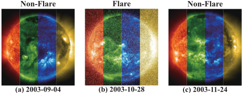
Stellar flares are defined as the rapid release of magnetic field energy stored in a star's atmosphere, as illustrated in Figure 1. These phenomena are crucial for understanding stellar structure, evolution, and magnetic activity, as well as exploring potentially habitable exoplanets and extraterrestrial life [Yong and Lin, 2024]. Flare records are currently obtained through continuous scanning of stars using survey telescopes in conjunction with manual analysis. Despite these efforts, the quantity of observed flare samples remains limited, rendering them inadequate for comprehensive research needs. Consequently, forecasting stellar flare timing holds significant importance for astronomical studies. However, to date, there has been no published research addressing this area.
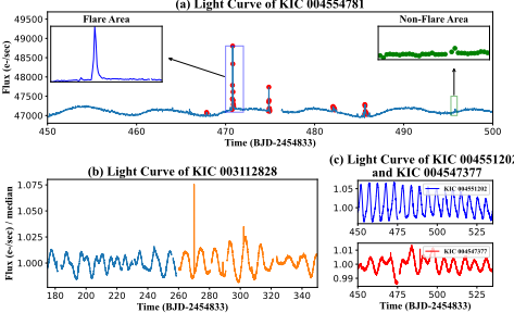
Solar flare prediction has garnered significant research attention [Deshmukh et al., 2022; Abduallah et al., 2023; Wen et al., 2023], but stellar flare forecasting presents distinct challenges compared to solar flare prediction. Leveraging the solar proximity, researchers can easily obtain solar magnetograms and magnetic field parameters, facilitating accurate solar flare predictions. In contrast, stellar flare forecasting predominantly relies on light curves. As depicted in Figure 2, a light curve represents the chronological variation of a stellar luminosity, measured in flux using Julian Date as the time axis. This figure illustrates that light curves often have missing data points. Additionally, two key characteristics emerge from the analysis: (1) A single star exhibits varying trend patterns across different time periods (refer to Figure 2(b)). (2) The variation trends differ significantly among different stars (see Figure 2(c)). These complex variations in light curves pose challenges for flare forecasting. Observably, a flare event is characterized by a rapid flux increase followed by a gradual decline, resulting in sharp short-term flux changes. Conversely, non-flare regions do not display such characteristics (as shown in Figure 2(a)).
The stellar flare forecasting task focuses on using light curves to predict whether a specified star will experience a flare within the next 24 hours. This can be viewed as a multitask framework that combines both forecasting and classification objectives. Deep learning methods [Zeng et al., 2023; Zhou et al., 2021] have been widely applied to time series analysis with promising results. However, these methods still do not demonstrate superior feature extraction capabilities compared to pre-trained large multi-modal models in stellar flare forecasting. The intrinsic characteristics of stars, their varying evolutionary stages, and external factors such as other celestial bodies and interstellar dust can lead to diverse patterns in light curves. These external influences make achieving high accuracy in stellar flare forecasting using only light curves particularly challenging. As a result, additional data sources are required to improve the reliability of predictions.
In this paper, we introduce a novel task of forecasting stellar flare events. To address this challenge, we propose the FLARE framework (Forecasting Light-curve-based Astronomical Records via feature Ensemble). Through empirical analysis, we observe that stellar flares exhibit strong correlations with various stellar physical properties. Consequently, FLARE incorporates these stellar features as auxiliary inputs to enhance light curve feature extraction and improve forecasting performance. Furthermore, our investigation reveals that frequent historical flare events are positively correlated with the likelihood of future flares. To leverage this temporal dependency, FLARE integrates historical flare records as additional auxiliary features for enhanced prediction accuracy. We also introduce two novel components: the Soft Prompt Module, which combines stellar physical feature names and values to facilitate star-specific feature detection, and the Residual Record Fusion Module, designed to integrate light curves with historical flare records for improved model robustness. Finally, we employ a large multi-modal model fine-tuned using LoRA [Hu et al., 2022] to extract features from the outputs of these modules, thereby enabling accurate stellar flare forecasting.
The main contributions are as follows: (1) We present the first attempt at developing a method for stellar flare forecasting, addressing a previously unexplored challenge in astrophysics. (2) Through rigorous experimental analysis, we demonstrate that both stellar physical properties and historical flare records play significant roles in flare forecasting. Then, we propose a large-scale model called FLARE, which has shown remarkable effectiveness in enhancing accuracy. (3) Extensive experimental results validate the superior performance of FLARE compared to other approaches.
2 Literature Review
2.1 Time Series Representation Learning
Inspired by the efficient performance of autoregressive models, MLPs such as DLinear [Zeng et al., 2023] demonstrate excellent performance. However, these methods often require additional design to capture time-wise dependency effectively. RNNs [Lai et al., 2018] are naturally suitable for modeling sequential data, while they suffer from issues such as gradient vanishing and struggle to learn relationships between multivariate variables. CNNs, unlike RNNs, are less prone to gradient vanishing and excel at capturing the local patterns in time series. However, they often require stacking multiple convolutional layers to learn global futures, as seen in TCN [Bai et al., 2018], which results in a significant training time cost. GNNs [Wu et al., 2020; Li et al., 2018] abstract variables as nodes and establish edges between multivariate variables, learning spatial dependencies through GCN [Kipf and Welling, 2017]. However, this approach relies on message passing to capture global features, and shows less scalable than Transformers. Leveraging the self-attention mechanism, Transformers are particularly adept at learning long-term temporal dependencies and complex multivariate correlations. Point-wise methods [Woo et al., 2022] learn correlations between time steps but become computationally expensive for long sequences. Series-wise methods [Liu et al., 2024b] pay attention to model multivariate dependencies by tokenization, but struggle with complex temporal patterns. Patch-wise methods [Nie et al., 2023; Zhang and Yan, 2023] adjust patch sizes for flexibility across different time series, making them more adaptable to different types of time series data. These methods have demonstrated certain advantages in specific tasks, and our work also adopts a patch-based approach in light curve processing.
2.2 Time Series Analysis based on PLMs
Among time series large models, aside from MOMENT [Goswami et al., 2024] and Chronos [Ansari et al., 2024] which are trained from scratch using big time series data, most approaches are adaptations of existing PLMs. These approaches can be sorted into three types:
Fine-tuning. Studies like UniTime [Liu et al., 2024a] and OFA [Zhou et al., 2023] unfreeze a portion of parameters, while others, including TEMPO [Cao et al., 2024] and LLM4TS [Chang et al., 2024] leverage Parameter-Efficient Fine-Tuning (PEFT) methods, such as LoRA [Hu et al., 2022], adapt to new data by increasing trainable parameters without disrupting the existing structure of the large model.
Alignment. PLMs trained on text data need to be aligned with time series data in the same data space. Based on the object of modification, these approaches can be divided into two categories. The first approach fine-tunes PLMs with time series data to map the model parameters into time series data space, as seen in LLM4TS [Chang et al., 2024]. The other approach maps the time series vector into text space, as demonstrated in TIME-LLM [Jin et al., 2024], which employs multi-head attention mechanisms to achieve mapping.
Prompt-learning. Studies such as UniTime [Liu et al., 2024a] incorporate text prompts, while TEST [Sun et al., 2024] employs the combination of trainable vectors and textual token embeddings to improve performance.
Although these methods generally perform well on specific tasks, they struggle to simultaneously handle multi-task time series analysis and text feature extraction.
3 Preliminaries
3.1 ProblemDefinition
The stellar flare forecasting task involves predicting whether a flare will occur in the future for a given star based on its light curve observations, physical properties, and historical flare records. For a star i, its physical properties are represented as P i = {(kim, vim)|m = 0, 1, . . . ,M}, where kim and vim are the name and the value of the m-th physical property, respectively. Here, kim is a text, while vim ∈ R ∪ {∅}, where ∅ indicates a missing value. The observed flux for star i at timestamp t is denoted as xit ∈ R ∪ {∅}. The historical flare records are represented by Ri = {(tisn , tien )|n = 0, 1, . . . , N}, where tisn and tien denote the start and end times of the n-th flare, respectively. A binary indicator variable is defined such that yi t = 1 if a flare occurs at timestamp t, i.e., if there exists a time t satisfying tisn < t < tien ; otherwise, yi t = 0. Additionally, yi (t0,t1) = 1 indicates that at least one flare occurred within the interval (t0, t1). Let K and H denote the observation window length and forecast horizon, respectively. The observed light curve is represented as ⃗xit = [xit-K , . . . , xit-1 ]⊤ ∈ RK , and the historical flare records are denoted by ⃗yi t = [yi t-K , . . . , yi t-1 ]⊤ ∈ RK . The forecast probability of a flare occurring between timestamps t and t′ = t + H - 1 is denoted by ˆ yi (t,t′ ) ∈ [0, 1]. The forecasting task can be formalized as follows:
where Φ represents the model parameters of the model F .
3.2 Experimental Observations
In Table 1, we present an experimental analysis to investigate how stellar physical properties and historical flare records influence the accuracy of flare forecasting using Kepler dataset.
Since stellar physical properties exhibit distinct characteristics compared to light curves, we first map these property values into a compatible dimensional space before concatenating them with the light curve data to derive forecast probabilities. For historical flare records, which share similar temporal characteristics with light curves, ⃗yi t and ⃗xit are concatenated along the flux dimension prior to model input.
The experimental results reveal that both stellar physical properties and historical flare records contribute meaningfully to forecasting performance. Furthermore, their combined use yields superior predictive accuracy compared to using either type of data alone. Interestingly, we observe that the marginal gain in performance diminishes after incorporating additional supplementary data. This finding suggests that stellar flare forecasting should not be approached solely as a time series prediction task based on light curves. Instead, leveraging both stellar physical properties and historical flare records represents an effective strategy for enhancing forecast accuracy and achieving a more comprehensive understanding of the underlying phenomena.
4 Methodology
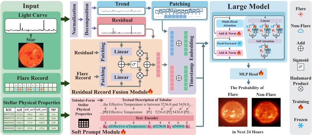
In this section, we present our proposed model, FLARE. The overall architecture of the model is illustrated in Figure 3, which comprises three key components. First, as detailed in Subsection 4.1, each light curve is decomposed into its trend and residual components, with historical flare records being integrated into the residual through a Residual Record Fusion Module to enhance robustness. Second, Subsection 4.2 introduces two prompt patterns based on tabular stellar physical properties and employs P-tuning [Liu et al., 2022b] to distinguish between different stars effectively. Finally, Subsection 4.3 describes the fine-tuning of PLM to simultaneously process text and light curves.
4.1 Light Curve Embedding
Typically, a flare only exists for a short period and is independent of the overall flux variation trend of the light curve. Furthermore, the periodic occurrence of flares only exists when the magnetic field of the star is stable. Given this phenomenon, separately handling the trend and the flare of the light curve could help eliminate mutual interference and improve light curve embedding. Even though the effectiveness of historical flare records has been verified in Subsection 3.2, fusing them with real flare could help improve robustness and reduce the misleading effect of false positive records. However, not all stars exhibit clear periodic luminosity variations. Moreover, their periods vary significantly, ranging from shorter than one day to longer than the observation window. In such cases, real-time embedding can be beneficial. Based on these considerations, we divide this subsection into three components: (1) normalization and decomposition, (2) trend processing and residual record fusion, and (3) timestamp embedding. As the light curve embedding process is uniform across stars, in the following text, we omit the superscript and use xt to represent the flux at timestamp t, and similarly for yt.
Normalization and Decomposition. Due to the inherent limitations in the precision of the telescope, flux values exhibit substantial variations across different observation periods. This variation necessitates the normalization of the data by dividing the flux values by the median, in order to effectively mitigate the potential influence of systematic errors. Besides, frequent data omissions in light curves require us to perform a decomposition that distinguishes the overall flux trend from local abrupt flux variations, while minimizing the impact of missing values. Given that the time steps with missing data are usually non-consecutive, we employ a moving average to capture the trend of the light curve's variations, explicitly excluding the missing data from the computation to ensure that the trend is not unduly influenced by data gaps. This process can be represented as:
| Light Curve | Light Curve + HFRs | Light Curve + SPPs | Light Curve + HFRs + SPPs | |||||
|---|---|---|---|---|---|---|---|---|
| Methods | Accuracy | F1 score | Accuracy | F1 score | Accuracy | F1 score | Accuracy | F1 score |
| PatchTST | 61.92 | 69.69 | 64.52 | 70.461 | 64.46 | 70.01 | 68.19 | 72.26 |
| iTransformer | 49.99 | 66.67 | 64.73 | 68.46 | 65.46 | 71.25 | 66.86 | 71.53 |
| Autoformer | 50.01 | 66.67 | 64.28 | 67.94 | 66.10 | 71.01 | 66.52 | 70.99 |
| Crossformer | 50.00 | 66.67 | 65.33 | 68.69 | 65.64 | 71.21 | 66.58 | 71.35 |
| ETSformer | 50.00 | 66.67 | 65.40 | 69.03 | 65.67 | 71.12 | 67.19 | 70.83 |
where ˆxj is the normalized xj, mj is an indicator for missing data, dW is the length of the sliding window, and xTj represents the trend at timestamp t. ⃗xTt = [xTt-K , · · · , xTt-1 ] ∈ RK are utilized to represent the trend of the light curve, with the rest representing the residual ⃗xRt = [xRt-K , · · · , xRt-1 ] ∈ RK , where xRj = ˆxj -xTj , j = t -K, · · · , t -1.
Trend Processing and Residual Record Fusion. Since both the trend ⃗xTt and the residual ⃗xRt are univariate time series, the temporal context at each timestamp plays a crucial role in data embedding. We generate patches for both the trend and the residual separately to obtain XT t ∈ RL×P and XR t ∈ RL×P , where L = ⌊ K-P S ⌋ is the number of patches with length of P , and S is the stride. The XT t is passed through the MLP to obtain the ˆXT t ∈ RL×d . For the residual, the gating mechanism is applied in conjunction with the flare record ⃗yt to process XR t . This process can be represented as:
where ˜W ∈ RP×d , {W gR,W gY ,W} ⊂ Rd×d , ˜b ∈ R2L, {bg , b} ⊂ RL. Yt is derived from ⃗yt by generating patches. ˆXR t ∈ RL×d is the embedding of the residual. σ denotes the sigmoid activation function and ⊙ represents Hadamard product, respectively.
Timestamp Embedding. As stars exist beyond the solar system, the time formatting used on Earth is not suitable and is typically represented by Julian Date, which is a continuous floating-point number. We extract the numerical values of each digit from the hundredths place to the ten-thousands place in a decimal manner, derive embeddings from these values, and use their sum as the timestamp embedding. Since the light curve has been divided into multiple patches, each patch requires a timestamp embedding. Given that the time intervals between adjacent time steps within the same patch are of fixed length, we employ the average timestamp embedding for the patch, and the collection of all patches is denoted as ET t ∈ RL×d . Following the three steps outlined above, the final time series embedding is obtained as XT S t = [ET t +XT t ;ET t +XR t ] ∈ R2L×d .
4.2 Prompt Design
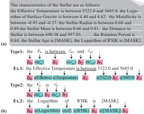
Motivation. Stellar flares are a prominent manifestation of stellar activity. As summarized in Yong [Yong and Lin, 2024]'s study, factors such as stellar age, rotation speed, and stellar mass are correlated with flare frequency, which further supports the use of stellar physical properties for flare forecast task. Stellar physical properties often exhibit frequent missing values and inconsistent numerical ranges. While interpolation and standardization can be used to address these issues separately, they may also introduce biases and lead to the loss of valuable physical information. Given that the physical properties of stars are presented as tabular data, and that Hegselmann [Hegselmann et al., 2023] has experimentally shown that combining column names with values leads to better performance than using only values, we organize the physical property values of stars along with their corresponding names into a textual structure. Furthermore, inspired by P-tuning [Liu et al., 2022b], we design the Soft Prompt Module to learn stellar physical properties for distinguishing stars.
Soft Prompt Module. The textual description of stellar physical properties is shown in Figure 4(a), where any physical property is represented as a range of values or an exact value. Inspired by P-tuning, which optimizes a small number of prompt embeddings and demonstrates good scalability while saving computational resources, we propose replacing part of the word vectors in the text with trainable parameters, as shown in Figure 4(b). We design corresponding replacement patterns based on the types of the physical property. In both pattens, two vectors (h0, h1) are retained to represent the start and end of a the physical property description, with a vector h1 separating the physical name from the value. Depending on the type of the physical property, an additional feature separator vector h2 will be inserted. All words except the replaced ones are embedded by the text encoder. Additionally, trainable embedding is utilized to represent the ID of the star. Through this prompt design, the meaning of physical property names, as well as the physical significance of their numerical value ranges, are both preserved. Finally, we use Xip ∈ RS×d to represent the embedding of the physical properties of the star i, and S is the number of tokens in the segmented textual descriptions.
4.3 Pre-Trained Large Model Fine-tuning
Zhou [Zhou et al., 2023] gives experimental evidence that training PLMs from scratch harms performance, while freezing most parameters and training only a small subset preserves the representational learning ability of PLMs. We freeze the majority of the parameters, particularly those in the multi-head attention mechanism and the feed forward layers, allowing the large model to fine-tune only the LayerNorm layers. To adapt to cross-modal inputs, we employ Low-Rank Adaptation (LoRA) [Hu et al., 2022] to introduce trainable low-rank matrices to the multi-head mechanism, which allows effective learning of the correlation between the physical property text vectors Xip ∈ RS×d and the light curve patches XT S t while introducing only a small number of trainable parameters. The final embedding Z i t = PLM(Xip ;XTS t ) ∈ R2L×d is obtained at the end of this process.
4.4 Loss Function
Since a portion of samples are false positives, label smoothing is applied. After computing forecast flare probabilities with the MLP, we use the cross-entropy loss function with label smoothing, which can be represented as:
where ϵ is the smoothing coefficient of the label, Ns denotes the number of stars, Ni represents the number of samples for star i, W c ∈ R1×2 , bc ∈ R1 , and POOLING refers to the operation of dimensionally reduction of Z i t .
5 Experiments
In this section, experiments are conducted to evaluate the effectiveness of FLARE and the indispensability of each module, and an analysis of flare forecasting cases is presented.
5.1 Experimental Setup
Datasets. Kepler mission [Borucki, 2016] monitored the luminosity variations of over 150,000 stars from 2009 to 2018. For our study, we select high-precision light curves of 7,160 stars with flare events from 2009 to 2013, sampled every halfhour intervals, forming the Kepler light curve dataset. Each observation window consists of 512 data points, and the object is to forecast whether a flare event will occur within the next 24 hours, corresponding to 48 data points. The light curves of each star are split into training and test sets in a 4:1 ratio based on chronological order, and the flare rate of the test set is controlled at 50% through random sampling.
Baselines. We compare the proposed method with five type baselines: (1) PLMs (MOMENT [Goswami et al., 2024], Chronos [Ansari et al., 2024], OFA [Zhou et al., 2023], and UniTime [Liu et al., 2024a]) (2) MLPs (Dlinear [Zeng et al., 2023], TiDE [Das et al., 2023], and FreTS [Yi et al., 2023]), (2) RNNs (GRU [Dey and Salem, 2017] and LSTNet [Lai et al., 2018]), (3) CNNs (MICN [Wang et al., 2023], TCN [Bai et al., 2018], and SCINet [Liu et al., 2022a]), (4) Transformers (PatchTST [Nie et al., 2023], iTransformer [Liu et al., 2024b], Autoformer [Wu et al., 2021], Crossformer [Zhang and Yan, 2023], ETSformer [Woo et al., 2022], and Informer [Zhou et al., 2021]).
Evaluation Metrics. To evaluate our forecasting model, we employ five evaluation metrics: AUC, Accuracy, Recall, F1 score and Precision. We prioritize high Recall and Accuracy while keeping adequate Precision for accurate forecasting.
Experiment Settings. We use AdamW [Loshchilov and Hutter, 2019] with a learning rate of 1e-5 as the optimizer, train for 200 epochs, and apply early stopping with a patience of 15. The PLMs, LSTNet, and TCN use publicly available code from their original papers, while the MLPs, Transformers, MICN, and SCINet use the code provided by TSLib 1 . Both the text encoder and the PLM are BERT [Devlin et al., 2019].
5.2 Performance Comparison
We compare FLARE with various baselines, conducting at least three runs to compute the average performance, as depicted in Table 2. Here, FLARE clearly outperforms other methods and is the only one achieving an accuracy greater than 70%. The following are three key observations:
(1) Among the five types of baselines, PLMs and RNNs typically perform well when neither historical flare records nor stellar physical properties are employed. The effectiveness of MOMENT and Chrones can be attributed to the knowledge gleaned from pre-trained large time-series models. We further analyze the subpar performance of OFA, which results from its simplistic approach to light curve processing. In contrast, UniTime, based on the same PLM, performs commendably. Additionally, the strong performance of RNNs is ascribed to the temporal characteristics of light curves.
1 https://github.com/thuml/Time-Series-Library
(2) Among MLPs and Transformers, only TiDE and PatchTST show classification ability when restricted to using only light curves. An analysis of this phenomenon is presented. The robust performance of TiDE is credited to the Residual Block, which bolsters its resilience and enables it to manage a certain level of noisy samples in the dataset. Among Transformers, point-wise methods (e.g., Autoformer and ETSformer) perform poorly, presumably because flux values lack contextual information, rendering them inadequate for effective feature learning at each time step. Serieswise methods (e.g., iTransformer) have difficulty capturing complex temporal dependencies, while patch-wise methods, such as PatchTST, exhibit excellent performance. Although Crossformer, also a patch-wise method, shows poor metrics, our analysis indicates that this is due to the mismatch between the univariate light curve and the Cross-Dimension Attention. (3) The inclusion of historical flare records and stellar physical properties improves the performance of all baselines, with only minor metric differences. This result underscores the significance of historical flare records and stellar physical properties in stellar flare prediction.
5.3 Ablation Study
Effectiveness of Each Module An ablation study is conducted to assess the effectiveness of each module within FLARE. Results in Table 3 show individual removal or replacement of modules. "FLARE w/o Soft Prompt Module" replaces its generated vector with one mapped from stellar physical property values. "FLARE w/o Residual Record Fusion Module" removes the module, concatenating historical flare records with the light curve along the flux dimension. "FLARE w/o LoRA" excludes LoRA during fine-tuning.
Our evaluation shows removing any of the three modules reduces specific performance metrics, while FLARE maintains robust performance across all metrics. Notably, omitting the Soft Prompt Module causes a significant performance drop, aligning with Hegselmann [Hegselmann et al., 2023], which states textual headers aid tabular data classification. Removing LoRA slightly decreases all five metrics, confirming its value in fine-tuning. Although removing the Residual Record Fusion Module causes minimal performance change, retaining it improves Recall, highlighting the module's effectiveness.
5.4 Case Study
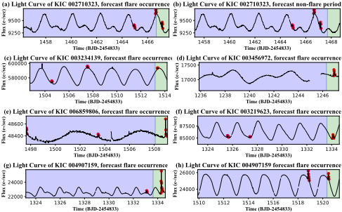
To elucidate the reasons underlying FLARE's flare forecasting capabilities, we conduct a case study to explore the working mechanism of FLARE. The forecast results of FLARE for selected samples are visualized in Figure 5. Evidently, FLARE can generate effective forecasts based on the observation area and can adapt to different stars and diverse flux variation patterns. Specifically, Figure 5(g) and Figure 5(h) demonstrate that FLARE can accurately predict flares on light curves with distinct flux variation patterns originating from the same star, highlighting its robust forecasting ability.
6 Conclusion
In this paper, we demonstrate that both stellar physical properties and historical flare records are beneficial for forecasting stellar flares. Hence, we propose the FLARE model, which incorporates two specialized modules: the Soft Prompt Module and the Residual Record Fusion Module. The Soft Prompt Module enables the model to differentiate between various star types, facilitating effective feature extraction tailored to each star's characteristics. Also, the Residual Record Fusion Module enhances model robustness by integrating historical flare records with light curve residuals. Experiments on the Kepler light curve dataset underscore FLARE's superior performance compared to existing models. We expect that these empirical results will provide valuable insights for future advancements in stellar flare forecast research.
| Methods | Light Curve | Methods | Light Curve + HFRs | ||||||
|---|---|---|---|---|---|---|---|---|---|
| Accuracy | F1 score | Recall | Precision | Accuracy | F1 score | + SPPs Recall | Precision | ||
| MOMENT | 62.65±0.40 | 70.02±0.04 | 87.25±0.77 | 58.48±0.40 | MOMENT∗ | 68.08±0.05 | 72.00±0.00 | 82.09±0.16 | 64.13±0.09 |
| Chronos | 61.26±0.43 | 69.49±0.45 | 88.09±1.05 | 57.34±0.42 | Chronos∗ | 65.01±0.31 | 70.88±0.08 | 85.08±0.82 | 60.71±0.40 |
| OFA | 49.99±0.00 | 66.66±0.00 | 99.99±0.00 | 50.00±0.00 | OFA∗ | 65.47±0.34 | 70.24±0.08 | 81.50±0.76 | 61.72±0.44 |
| UniTime | 61.45±2.07 | 69.42±0.65 | 87.44±2.44 | 57.64±1.89 | UniTime∗ | 67.43±0.20 | 71.83±0.15 | 83.06±0.90 | 63.28±0.35 |
| DLinear | 50.00±0.00 | 66.66±0.00 | 99.99±0.00 | 50.00±0.00 | DLinear∗ | 66.04±0.22 | 71.18±0.03 | 83.87±0.66 | 61.83±0.31 |
| TiDE | 59.43±0.25 | 68.64±0.04 | 88.80±0.62 | 55.95±0.22 | TiDE∗ | 66.04±0.73 | 71.14±0.02 | 83.71±1.72 | 61.89±0.97 |
| FreTS | 49.99±0.00 | 66.66±0.00 | 99.99±0.00 | 49.99±0.00 | FreTS∗ | 65.64±0.48 | 70.25±0.04 | 81.12±1.10 | 61.96±0.66 |
| MICN | 49.99±0.00 | 66.66±0.00 | 99.99±0.00 | 50.00±0.00 | MICN∗ | 65.58±0.12 | 70.74±0.02 | 83.22±0.23 | 61.52±0.15 |
| TCN | OOT | OOT | OOT | OOT | TCN∗ | OOT | OOT | OOT | OOT |
| SCINet | OOT | OOT | OOT | OOT | SCINet∗ | 67.38±0.61 | 71.88±0.12 | 83.36±1.11 | 63.19±0.78 |
| GRU | 53.23±4.57 | 67.50±1.17 | 96.79±4.52 | 52.00±2.83 | GRU∗ | 66.54±0.63 | 71.14±0.04 | 82.49±1.54 | 62.57±0.87 |
| LSTNet | 60.05±0.58 | 68.69±0.06 | 87.67±1.16 | 56.48±0.51 | LSTNet∗ | 67.84±0.45 | 71.55±0.15 | 80.88±1.52 | 64.17±0.77 |
| PatchTST | 62.09±0.19 | 69.74±0.04 | 87.40±0.33 | 58.02±0.18 | PatchTST∗ | 68.40±0.29 | 72.29±0.05 | 82.48±0.08 | 64.38±0.46 |
| iTransformer | 50.00±0.00 | 66.66±0.00 | 99.99±0.00 | 50.00±0.00 | iTransformer∗ | 66.30±0.53 | 70.81±0.09 | 81.74±1.18 | 62.47±0.72 |
| Autoformer | 49.99±0.00 | 66.66±0.00 | 99.99±0.00 | 50.00±0.00 | Autoformer∗ | 63.62±0.80 | 69.72±0.33 | 83.74±1.41 | 59.73±0.82 |
| Crossformer | 50.00±0.00 | 66.66±0.00 | 99.99±0.00 | 50.00±0.00 | Crossformer∗ | 66.66±0.46 | 71.19±0.05 | 82.37±0.94 | 62.69±0.61 |
| ETSformer | 50.00±0.00 | 66.66±0.00 | 99.99±0.00 | 50.00±0.00 | ETSformer∗ | 66.46±0.16 | 70.73±0.25 | 81.05±1.06 | 62.75±0.30 |
| Informer | 52.93±4.13 | 67.38±1.00 | 96.97±4.28 | 51.78±2.51 | Informer∗ | 65.42±0.30 | 70.45±0.03 | 82.42±0.65 | 61.51±0.38 |
| - | - | - | - | - | FLARE | 71.65±0.35 | 74.11±0.02 | 81.11±1.04 | 68.22±0.72 |
| Method | AUC | Accuracy | F1 score | Recall | Precision |
|---|---|---|---|---|---|
| FLARE w/o Soft Prompt Module | 77.47 | 67.47 | 71.55 | 81.79 | 63.58 |
| FLARE w/o Residual Record Fusion Module | 79.22 | 71.80 | 74.11 | 80.73 | 68.50 |
| FLARE w/o LoRA | 79.45 | 71.37 | 73.91 | 81.11 | 67.89 |
| FLARE | 79.89 | 71.65 | 74.11 | 81.11 | 68.22 |
Acknowledgments
This work was supported in part by the National Key R&D Program of China(No. 2022ZD0160601), Strategic Priority Research Program of Chinese Academy of Sciences under Grant XDA0480404, Beijing Municipal Science and Technology Project (Z231100007423004), and National Natural Science Foundation of China (No. 62276260, 62472423).
Contribution Statement
Bingke Zhu and Xiaoxiao Wang contributed equally to this work. Yingying Chen and Jinqiao Wang are the corresponding authors.
@inproceedings{ijcai2025p1056,
  title     = {FLARE: A Framework for Stellar Flare Forecasting Using Stellar Physical Properties and Historical Records},
  author    = {Zhu, Bingke and Wang, Xiaoxiao and Jia, Minghui and Tao, Yihan and Kong, Xiao and Luo, Ali and Chen, Yingying and Tang, Ming and Wang, Jinqiao},
  booktitle = {Proceedings of the Thirty-Fourth International Joint Conference on
               Artificial Intelligence, {IJCAI-25}},
  publisher = {International Joint Conferences on Artificial Intelligence Organization},
  editor    = {James Kwok},
  pages     = {9501--9509},
  year      = {2025},
  month     = {8},
  note      = {AI4Tech: AI Enabling Technologies},
  doi       = {10.24963/ijcai.2025/1056},
  url       = {https://doi.org/10.24963/ijcai.2025/1056},
}
TY - CPAPER TI - FLARE: A Framework for Stellar Flare Forecasting Using Stellar Physical Properties and Historical Records AU - Zhu, Bingke AU - Wang, Xiaoxiao AU - Jia, Minghui AU - Tao, Yihan AU - Kong, Xiao AU - Luo, Ali AU - Chen, Yingying AU - Tang, Ming AU - Wang, Jinqiao T2 - Proceedings of the Thirty-Fourth International Joint Conference on Artificial Intelligence, IJCAI-25 PB - International Joint Conferences on Artificial Intelligence Organization PY - 2025 SP - 9501 EP - 9509 DO - 10.24963/ijcai.2025/1056 UR - https://doi.org/10.24963/ijcai.2025/1056 ER -Copied
Machine-readable versions of this paper, for tools and AI agents:





