
Faster Annotation for Elevation-Guided Flood Extent Mapping by Consistency-Enhanced Active Learning
Proceedings of the Thirty-Fourth International Joint Conference on Artificial Intelligence. AI and Social Good. Pages 9511-9519.
https://doi.org/10.24963/ijcai.2025/1057
Keywords
- Computer Vision: General
- Machine Learning: General
Abstract
Flood extent mapping is crucial for disaster response and damage assessment. While Earth imagery and terrain data (in the form of DEM) are now readily available, there are few flood annotation data for training machine learning models, which hinders the automated mapping of flooded areas. We propose ALFA, an interactive active-learning-based approach to minimize the annotators' efforts when preparing the ground-truth flood map in a satellite image. ALFA calibrates the prediction consistency of a segmentation model (1) across training cycles and (2) for various data augmentations. The two consistencies are integrated into the design of both the acquisition function and the loss function to enhance the robustness of active learning with limited annotation inputs. ALFA recommends those superpixels that the underlying model is most uncertain about, and users can annotate their pixels with minimal clicks with the help of elevation guidance. Extensive experiments on various regions hit by flooding show that we can improve the annotation time from hours to around 20 minutes. ALFA is open sourced at https://github.com/saugatadhikari/alfa.
- [Achanta et al., 2012] Radhakrishna Achanta, Appu Shaji, Kevin Smith, Aurélien Lucchi, Pascal Fua, and Sabine Süsstrunk. SLIC superpixels compared to state-of-the-art superpixel methods. IEEE Trans. Pattern Anal. Mach. In- tell., 34(11):2274-2282, 2012.
- [Adhikari et al., 2022] Saugat Adhikari, Da Yan, Mirza Tanzim Sami, Jalal Khalil, Lyuheng Yuan, Bhadhan Roy Joy, Zhe Jiang, and Arpan Man Sainju. An elevation-guided annotation tool for flood extent mapping on earth imagery. In SIGSPATIAL. ACM, 2022.
- [Adhikari et al., 2025] Saugat Adhikari, Da Yan, Tianyang Wang, Landon Dyken, Sidharth Kumar, Lyuheng Yuan, Akhlaque Ahmad, Jiao Han, Yang Zhou, and Steve Petruzza. Faster annotation for elevation-guided flood extent mapping by consistency-enhanced active learn- ing. https://github.com/saugatadhikari/alfa/blob/main/ appendix.pdf, 2025. Accessed: 2025-05-14. Link
- [Bastani et al., 2023] Favyen Bastani, Piper Wolters, Ritwik Gupta, Joe Ferdinando, and Aniruddha Kembhavi. Sat- laspretrain: A large-scale dataset for remote sensing im- age understanding. In ICCV, pages 16726-16736. IEEE, 2023.
- [Bonafilia et al., 2020] Derrick Bonafilia, Beth Tellman, Tyler Anderson, and Erica Issenberg. Sen1floods11: a georeferenced dataset to train and test deep learning flood algorithms for sentinel-1. In CVPR, pages 835-845. Com- puter Vision Foundation / IEEE, 2020.
- [Cong et al., 2022] Yezhen Cong, Samar Khanna, Chenlin Meng, Patrick Liu, Erik Rozi, Yutong He, Marshall Burke, David B. Lobell, and Stefano Ermon. Satmae: Pre-training transformers for temporal and multi-spectral satellite im- agery. In NeurIPS, 2022.
- [Dai et al., 2020] Chengliang Dai, Shuo Wang, Yuanhan Mo, Kaichen Zhou, Elsa D. Angelini, Yike Guo, and Wen- jia Bai. Suggestive annotation of brain tumour images with gradient-guided sampling. In MICCAI, volume 12264 of Lecture Notes in Computer Science, pages 156-165. Springer, 2020.
- [den Bergh et al., 2015] Michael Van den Bergh, Xavier Boix, Gemma Roig, and Luc Van Gool. SEEDS: superpix- els extracted via energy-driven sampling. Int. J. Comput. Vis., 111(3):298-314, 2015.
- [Dyken et al., 2024] Landon Dyken, Saugat Adhikari, Pravin Poudel, Steve Petruzza, Da Yan, Will Usher, and Sidharth Kumar. Enabling quick, accurate crowdsourced annotation for elevation-aware flood extent mapping, 2024.
- [Golestaneh and Kitani, 2020] S. Alireza Golestaneh and Kris Kitani. Importance of self-consistency in active learn- ing for semantic segmentation. In BMVC. BMVA Press, 2020.
- [He et al., 2022] Kaiming He, Xinlei Chen, Saining Xie, Yanghao Li, Piotr Dollár, and Ross B. Girshick. Masked autoencoders are scalable vision learners. In CVPR, pages 15979-15988. IEEE, 2022.
- [Hong et al., 2024] Danfeng Hong, Bing Zhang, Xuyang Li, Yuxuan Li, Chenyu Li, Jing Yao, Naoto Yokoya, Hao Li, Pedram Ghamisi, Xiuping Jia, Antonio Plaza, Paolo Gamba, Jón Atli Benediktsson, and Jocelyn Chanussot. Spectralgpt: Spectral remote sensing foundation model. IEEE Trans. Pattern Anal. Mach. Intell., 46(8):5227-5244, 2024.
- [Huang et al., 2024] Siyu Huang, Tianyang Wang, Haoyi Xiong, Bihan Wen, Jun Huan, and Dejing Dou. Tem- poral output discrepancy for loss estimation-based active learning. IEEE Trans. Neural Networks Learn. Syst., 35(2):2109-2123, 2024.
- [Jakubik et al., 2023] Johannes Jakubik, Sujit Roy, C. E. Phillips, Paolo Fraccaro, Denys Godwin, Bianca Zadrozny, Daniela Szwarcman, Carlos Gomes, Gabby Nyirjesy, Blair Edwards, Daiki Kimura, Naomi Simumba, Linsong Chu, S. Karthik Mukkavilli, Devyani Lambhate, Kamal Das, Ranjini Bangalore, Dario Oliveira, Michal Muszynski, Kumar Ankur, Muthukumaran Ramasub- ramanian, Iksha Gurung, Sam Khallaghi, Hanxi, Li, Michael Cecil, Maryam Ahmadi, Fatemeh Kordi, Hamed Alemohammad, Manil Maskey, Raghu Ganti, Kommy Weldemariam, and Rahul Ramachandran. Foundation models for generalist geospatial artificial intelligence, 2023.
- [Lenczner et al., 2022] Gaston Lenczner, Adrien Chan-Hon- Tong, Bertrand Le Saux, Nicola Luminari, and Guy Le Besnerais. DIAL: deep interactive and active learning for semantic segmentation in remote sensing. IEEE J. Sel. Top. Appl. Earth Obs. Remote. Sens., 15:3376-3389, 2022.
- [Matgen et al., 2020] Patrick Matgen, Sandro Martinis, Wolfgang Wagner, Vahid Freeman, Peter Zeil, Niall Mc- Cormick, et al. Feasibility assessment of an automated, global, satellite-based flood-monitoring product for the copernicus emergency management service. Luxembourg: Publications Office of the European Union, 2020.
- [NCSU, 2023] NCSU. NCSU Libraries. https://www.lib. ncsu.edu/gis/elevation, 2023. Link
- [NOAA, 2016] NOAA. Hurricane matthew imagery. https: //geodesy.noaa.gov/storm archive/storms/matthew/, 2016. (Accessed on 08/02/2023). Link
- [NOAA, 2017] NOAA. Hurricane harvey imagery. https://storms.ngs.noaa.gov/storms/harvey/index.html#7/ 28.411/-96.691, 2017. (Accessed on 08/02/2023). Link
- [Oddo and Bolten, 2019] PC Oddo and JD Bolten. The value of near real-time earth observations for improved flood disaster response. frontiers in environmental science, 2019.
- [Sami et al., 2024] Mirza Tanzim Sami, Da Yan, Saugat Ad- hikari, Lyuheng Yuan, Jiao Han, Zhe Jiang, Jalal Khalil, and Yang Zhou. Evanet: Elevation-guided flood extent mapping on earth imagery, 2024. IJCAI
- [Shin et al., 2021] Gyungin Shin, Weidi Xie, and Samuel Al- banie. All you need are a few pixels: semantic segmenta- tion with pixelpick. In ICCVW, pages 1687-1697. IEEE, 2021.
- [Siddiqui et al., 2020] Yawar Siddiqui, Julien Valentin, and Matthias Nießner. Viewal: Active learning with viewpoint entropy for semantic segmentation. In CVPR, pages 9430- 9440. Computer Vision Foundation / IEEE, 2020.
- [Sinha et al., 2019] Samarth Sinha, Sayna Ebrahimi, and Trevor Darrell. Variational adversarial active learning. In ICCV, pages 5971-5980. IEEE, 2019.
- [Tarvainen and Valpola, 2017] Antti Tarvainen and Harri Valpola. Mean teachers are better role models: Weight- averaged consistency targets improve semi-supervised deep learning results. In NIPS, pages 1195-1204, 2017. [USGS, 2023] USGS. Tnm download v2. https:// apps.nationalmap.gov/downloader/, 2023. (Accessed on 08/02/2023). Link
- [Wahlstrom et al., 2015] Margareta Wahlstrom, Debarati Guha-Sapir, et al. The human cost of weather-related disasters 1995-2015. Geneva, Switzerland: UNISDR, 2015.
- [Yang et al., 2017] Lin Yang, Yizhe Zhang, Jianxu Chen, Siyuan Zhang, and Danny Z. Chen. Suggestive annota- tion: A deep active learning framework for biomedical image segmentation. In MICCAI, volume 10435 of Lec- ture Notes in Computer Science, pages 399-407. Springer, 2017.
References were extracted automatically from the PDF and may contain errors.
Full text extracted automatically from the PDF; figures, tables and equations may differ. The PDF is the version of record.
1 Introduction
Climate change is drastically increasing the intensity and occurrence of floods [Matgen et al., 2020]. In the past two decades, flooding has negatively impacted over 2.3 billion people [Wahlstrom et al., 2015]. Therefore, accurate and timely mapping of flood extent is crucial for effectively planning rescue and rehabilitation efforts [Oddo and Bolten, 2019]. Thanks to the rapid advancement in AI and the abundant geospatial data collected, such as satellite imagery from NASA and ESA and digital elevation model (DEM) data from USGS, it is the right timing to harness them to improve the performance of flood extent mapping.
Although annotated natural images are abundant, most Earth imagery data are unannotated. A popular annotated dataset for flood mapping is Sen1Floods11 [Bonafilia et al., 2020] which was curated by a startup called 'Cloud to Street' (now Floodbase) but it is very small, and [Bonafilia et al., 2020] reports that models trained on Sen1Floods11 have a quite low test mean IoU for the water class.
Two solutions can improve the performance of flood mapping. One solution is to train a more advanced AI model with a larger annotated dataset, and this paper aims to facilitate the productivity of flood annotation with a new strategy to enable the curation of larger annotated datasets. The other solution is to fine-tune a large geo-foundation model pre-trained with a vast number of satellite images in a self-supervised manner, but the fine-tuning stage still requires an annotated dataset of reasonable size. In fact, NASA and IBM recently released a pioneering geo-foundation model called Prithvi [Jakubik et al., 2023], whose fine-tuning on Sen1Floods11 has significantly improved the performance of flood mapping as compared with the results by training a model from scratch on Sen1Floods11 [Bonafilia et al., 2020].
In this paper, we propose to facilitate the annotation of more satellite imagery (e.g., via crowdsourcing) by designing a novel flood annotation tool based on active learning. Given a large pool of unlabeled data, active learning (AL) minimizes the amount of data to be labeled to train an underlying machine learning model, in order to yield a comparable performance as if using much more labeled data. AL operates in cycles: in each cycle, the most informative or valuable data points are selected for labeling (through an acquisition function) and then the model gets retrained. Our use of AL is different from conventional methods since:
- ÷ Conventional AL minimizes the annotation cost since finding an expert to annotate each data point is expensive, but there is no time restrictions. In contrast, we allow non-experts to annotate satellite images but we aim to minimize the annotation time; retraining should be fast to support interactive user annotating, so the underlying model should be lightweight.
- ÷ The problem domain in convention AL is the entire dataset, from which a small subset of data items are selected for user annotation. In contrast, our problem domain is each individual satellite image, wherein informative regions are selected for annotation. For different satellite images, the underlying model can be the same while the trained model parameters can be different.
- ÷ The end goal of conventional AL is the trained underlying model, but our end goal is annotating each image while the underlying model is just used to automatically label each pixel as 'flooded' or 'dry' (trained based on users' limited annotations), so it is desirable to overfit the underlying model (e.g., a lightweight U-Net variant) on the current image to minimize annotation efforts and improve annotation quality. The annotated images are collected usually to collectively train or fine-tune a more powerful model, such as a geo-foundation model often based on masked autoencoder (MAE) [He et al., 2022].
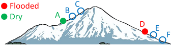
Besides active learning, we also utilize terrain guidance as illustrated in Figure 1 to improve the productivity and quality of flood annotation, as elevation data can be readily obtained from the digital elevation model (DEM) data downloadable from USGS [USGS, 2023].
The end product is an annotation tool called Active Learning for Flood Annotation (ALFA), which is open sourced at https://github.com/saugatadhikari/alfa. Our annotation tool takes the satellite image of a flooded area along with its associated elevation map (from DEM data), and visualizes the terrain in 3D. The tool supports rotation, movement, zoom-in and zoom-out of the terrain, so that users can annotate the pixels in red (to mean 'flooded') or blue (to mean 'dry') from different views. Elevation-guided breadth-first search (BFS) [Adhikari et al., 2022] is adopted to speed up annotation, where (i) when an annotator marks an individual pixel p as flooded, the label propagates to nearby pixels with lower elevations by 'pit-filling' BFS stopping when reaching pixels with elevation higher than that of p, and (ii) when an annotator marks an individual pixel as dry, the label propagates to nearby pixels by 'hill-climbing' BFS stopping when reaching pixels with elevation starting to drop. The labels of some pixels covered by tree canopy may be derived in this way from nearby pixels using the physical law of gravity.
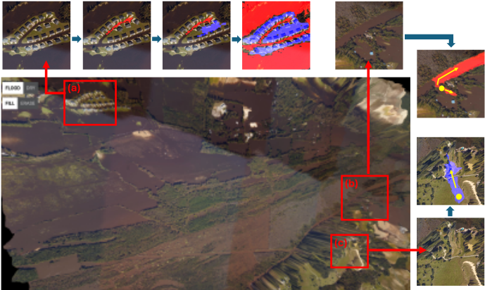
Figure 2 shows the upper-left portion of our tool's interface from a particular view, and more elements of the interface will be introduced later in Figure 3 when we introduce our AL-based annotation pipeline. Figure 2(a) shows an area with many houses that are partitioned into multiple islands due to flooding, and such areas would need very careful and fine-grained user annotations with many flood/dry clicks, so directly annotating an entire satellite image is very timeconsuming, typically hours even for domain experts. Figures 2(b) and (c) show how the elevation-guided BFS can automatically label many pixels after just one click.
Our main contributions are summarized as follows:
- ÷ To keep the number of region candidates tractable (for computing acquisition functions), ALFA recommends superpixels (wherein pixels tend to have the same label) rather than individual pixels for annotation, but users can
- utilize elevation guidance to click on only a few pixels to cover many pixels with their labels automatically derived, including those outside the recommended superpixels.
- ÷ We identify two label-free consistency metrics that can guide active learning: (1) view consistency, which states that if the label prediction of a pixel changes with data augmentation, then it is more informative for annotation to retrain the underlying model; (2) temporal consistency, which states that if the output of the underlying model at a pixel location changes a lot across different cycles, then it is more informative for annotation. Both consistency metrics are integrated into the design of our acquisition function and loss function, and our solution is applicable to active learning in general (not specific to flood mapping) if we replace pixels with data items.
- ÷ Our acquisition function not only integrates the confidence (e.g., measured by entropy) and consistencies, but also considers a 'tree score' specific to our flood annotation domain to minimize the probability that regions covered by tree canopy get recommended (since they are ambiguous and users cannot give labels properly).
- ÷ We conduct extensive studies to verify that ALFA can significantly improve the annotation productivity and quality. ALFA is open sourced at https://github.com/ saugatadhikari/alfa.
2 RelatedWork
Due to page limit, we only briefly mention the related work. Appendix A online [Adhikari et al., 2025] gives more details.
Superpixel Algorithms. A superpixel is a group of contiguous pixels that share almost the same color, and representative algorithms include SLIC [Achanta et al., 2012] and SEEDS [den Bergh et al., 2015]. We adopt SEEDS since it generates higher quality superpixels than SLIC and is faster [den Bergh et al., 2015].
Image-based Active Learning. The image-based AL for semantic segmentation considers an entire image as the basic unit to be recommended for annotation. Related works include [Dai et al., 2020], [Sinha et al., 2019], [Yang et al., 2017] and [Huang et al., 2024]. All these works recommend entire images for annotation which is different from our setting where we recommend regions inside an image.
Region-based Active Learning. The region-based AL for semantic segmentation divides each image into nonoverlapping local regions and recommends regions for annotation. Some works divide the image into uniform patches for recommendation, such as EquAL [Golestaneh and Kitani, 2020] and DIAL [Lenczner et al., 2022]. However, a patch may contain pixels from different classes, so it is not an ideal unit for annotation. PixelPick [Shin et al., 2021] recommends sparse pixels for annotation based on uncertainty sampling using entropy measures. This method is inferior to ours since we recommend region units with label homogeneity, and each click can label many pixels (by elevation-guided BFS) to reduce the time to annotate a satellite image. To our knowledge, ViewAL [Siddiqui et al., 2020] is the only work that recommends superpixels. It studies the segmentation of 3D objects in multi-view datasets by enforcing that the same surface point in a scene should receive the same label when observed from different viewpoints. In contrast, we target a satellite image associated with a land surface derived from DEM data, rather than 3D objects in a multi-view dataset.
Geo-foundation Models. Recently, several geo-foundation models have been proposed based on MAE to pre-train with the vast amount of unannotated satellite imagery, such as Prithvi [Jakubik et al., 2023], SatMAE [Cong et al., 2022] and SpectralGPT [Hong et al., 2024]. The self-supervision during pre-training is achieved by masking out a fraction of patches for recovery. Our annotated images can be used to fine-tune these geo-foundation models.
3 Methodology
We regard each satellite image as a 2D grid I of size H ⇥W, and denote a pixel by p = (x, y), where x and y are the pixel coordinates in I. We also assume that an elevation map h(I) is available, and the elevation of pixel p is h(p). Our AL framework uses EvaNet [Sami et al., 2024] as the underlying segmentation model, which is a U-Net variant that (1) uses (de)convolution operations which integrates the elevation map h by a location-sensitive gating mechanism to regulate how much spectral features flow through adjacent layers, and that (2) uses a loss function Leva which intergates the physical rule that if a location is flooded (resp. dry), then its adjacent locations with a lower (resp. higher) elevation must also be flooded (resp. dry). We use EvaNet due to its lightweight training workload and its capability to utilize the elevation map to improve segmentation quality, and please refer to [Sami et al., 2024] for its detailed design.
Since EvaNet takes an input image of size 128 ⇥ 128, we partition I into 128 ⇥ 128 patches as in [Sami et al., 2024] and each patch is passed through EvaNet for segmentation. The segmentation results of all patches can be stitched back to obtain the segmentation results of the entire I.
Figure 3 overviews the workflow of ALFA, where the pretrained parameters of EvaNet are initially used, and the superpixels of I are precomputed using SEEDS [den Bergh et al., 2015]. In each AL cycle, each patch of I is passed through EvaNet to obtain an output tensor with 2 channels, one for 'flood' scores and the other for 'dry' scores. The results from all patches are stitched together to get a flood score map and a dry score map, both of size H ⇥W. Let the flood (resp. dry) score of a pixel p be sflood(p) (resp. sdry(p)), then a channel-wise softmax is conducted to normalize the score
maps into probability maps: pflood(p) = esflood(p) esflood(p)+esdry(p) (resp. pdry(p) = esdry(p) esflood(p)+esdry(p) ). The probability maps can
already be used to measure the confidence of model predictions to select the most uncertain superpixels for user annotation, but we can further improve the robustness of the uncertainty measure by considering view consistency and temporal consistency, which we will discuss in detail later.
As the lower-right corner of Figure 3 shows, the highuncertainty superpixels (highlighted in green) are recommended for user annotation, and users may click pixels within these superpixels to annotate with a 'flood' or 'dry' label. Since the label is propagated using elevation-guided BFS, the annotated pixels may propagate outside the recommended pixels. When a user finishes the annotation activities in the current cycle, it can click a "retrain" button so that the EvaNet will be retrained using all the annotated pixels so far, to be used by the next AL cycle. Note that (1) the loss function only considers annotated pixels for supervision, and it integrates both elevation guidance (i.e., Leva) and the consistency measures to improve training performance (we will discuss the details later), and that (2) the number of annotated pixels is small but increases after each cycle, so model retraining is very efficient with a GPU.
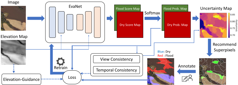
At any time during the annotation, users may visualize (1) the current prediction by EvaNet, (2) the recommended superpixels in the current cycle, and (3) all the annotated pixels so far, by clicking the corresponding button in the interface (or pressing the corresponding key on the keyboard) to facilitate annotation. Users are also allowed to erase old pixel annotations to fix annotation errors made previously.
We retrain for 3 epochs in each cycle, taking 80-120 seconds in total. To utilize the time during retraining, users can continue to annotate more pixels by comparing the previous EvaNet prediction and the satellite image to locate wrongly predicted pixels/regions to annotate with the correct labels.
In the sequel, we first introduce our consistency measures, then the acquisition function, and finally the loss function.
Pixel-level Uncertainty. Given the current predictions by the EvaNet model, we define the uncertainty score for each pixel. We consider three uncertainty measures: (1) confidence, (2) view consistency, and (3) temporal consistency, all defined based on the dry and flood probability maps.
For confidence, we consider two alternative measures based on probability offset and entropy, respectively:
Probability offset measures how much the flooding probability deviates from 0.5 (i.e., 50% flooding 50% dry). For uoff(p) (resp. uent(p)), the larger (resp. smaller) its value is, the more confident the EvaNet prediction is for p.
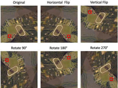
For view consistency, we penalize those pixels whose predictions vary with data augmentation. For each patch (i.e., input to EvaNet), we consider the 6 views (5 augmentations) as shown in Figure 4, all passed through EvaNet to get their probability maps. For a pixel p in the original patch, we denote the predicted flood (resp. dry) probability of its corresponding pixel in the ith view by p(i) flood (p) (resp. p(i) dry (p)), and denote the corresponding entropy by u(i) ent (p) as in Eq (2), then we can define the bias of p in the ith view in two alternative ways:
Based on our experiments (see Table 5 in Appendix C online [Adhikari et al., 2025]), b(i) ent performs better than b(i) prob when used to calculate view inconsistency, so we assume that b(i) ent is adopted from now on.
After we compute the biases in the 6 different views, we can aggregate them in two alternative ways:
which basically computes the variance of u(i) ent (p), and
which computes the maximum bias caused by data augmentation. Based on our experiments (see Table 6 in Appendix C [Adhikari et al., 2025]), ⇢max performs better when measuring view inconsistency, so we assume that ⇢max is adopted from now on.
For temporal consistency, we measure how much the predicted probabilities differ between two consecutive AL cycles:
where ♣c denotes the prediction in the cth cycle. As [Huang et al., 2024] shows, temporal output difference is an effective measure of model uncertainty about its prediction.
Besides these measures, we also consider the concept of 'tree score' to avoid recommending pixels covered by tree canopy, as their labels are hard to determine by human eyes. Specifically, we train a standard U-Net model (called as ForestNet) on satellite images carefully annotated with forest maps, and use it to predict the pixel-level forest pixel probabilities for our test regions. Let ptree(p) denote the tree probability score for pixel p by ForestNet, and let uconf be the confidence score that can be either uoff (Eq (1)) or -uent (Eq (2)), then the overall uncertainty score for p is:
where ⇢max(p) is the view inconsistency score defined in Eq (6), and utemp(p) is the temporal inconsistency score defined in Eq (7). Hyperparameters λ1, λ2 and λ3 balance the importance between the various uncertainty measures, and our goal is to recommend pixels with large u(p).
Superpixel-level Uncertainty Score Aggregation. Since ALFA recommends superpixels rather than pixels, we need to compute uncertainty score for each superpixel by aggregating the uncertainty scores of its pixels. Given superpixel S containing ♣S♣ pixels, we define its uncertainty score in two alternative ways, by average or maximum aggregation:
Based on our experiments (See Table 6 in Appendix C [Adhikari et al., 2025]), the average scheme works the better and is thus used by default. This is reasonable since averaging is more robust to noise. We recommend top-N superpixels for annotation by the users, and the default value of N is set to 25 which is observed to work well in our experiments.
Retraining by Semi-Supervised Learning. We retrain the EvaNet using (1) the supervised loss head Leva originally proposed in [Sami et al., 2024] that penalizes label predictions of pixel pairs that violate elevation guidance (e.g., a 'flooded' pixel with a nearby 'dry' pixel with a lower elevation), as well as (2) two unsupervised loss heads based on view consistency and temporal consistency, respectively.
Let the current AL cycle number be c, and let the set of all pixels not yet labeled by users be Uc, then both unsupervised loss heads are computed over pixels of Uc.
The view consistency loss of the current cycle is given by
which minimizes the prediction variance of every unlabeled pixel among the 6 different views.
Temporal consistency is enforced by minimizing the prediction difference between the current model at cycle c and a baseline model obtained by applying an exponential moving average (EMA) to the historical parameters as inspired by Mean Teacher [Tarvainen and Valpola, 2017]:
where wc-1 is the retrained EvaNet parameter at cycle (c - 1), w is the parameter of the baseline model, ↵ is the EMA decay rate, and Eq (12) updates w of cycle (c - 2) with the retrained parameter at cycle (c - 1). This design is found to perform better than minimizing the prediction difference at consecutive cycles c and (c - 1) [Huang et al., 2024].
Let us denote by utemp(p)♣EMA the sum of squared prediction differences as formulated in Eq (7) except that the model predictions at cycle (c - 1) is replaced by the predictions by the baseline model with parameter w. The temporal consistency loss at cycle c is hence given by
The overall loss objective at cycle c is hence given by:
where β1 and β2 are hyperparameters to balance loss terms.
4 Experiments
Datasets. We obtain high-resolution aerial imagery from NOAA NGS during Hurricane Matthew in North Carolina (NC) in 2016 [NOAA, 2016] and Hurricane Harvey in Texas (TX) in 2017 [NOAA, 2017] along with their accompanied DEM data. Table 1 summarizes our regions: R1-R4 are from Matthew 2016 and R5 is from Harvey 2017. The ground-truth annotations of these regions are obtained using the FloodTrace tool [Dyken et al., 2024], and some ambiguous pixels (e.g., those covered by tree canopies) are left unlabeled. See Appendix B [Adhikari et al., 2025] for more details.
| Method | Initial Metrics | Final Metrics | Dry | Flood | ||||||
|---|---|---|---|---|---|---|---|---|---|---|
| Accuracy | mIoU | Accuracy | mIoU | Precision | Recall | F1 score | Precision | Recall | F1 score | |
| Random Sampling | 98.92 | 97.57 | 98.99 | 97.69 | 98.33 | 98.89 | 99.52 | 99.20 | ||
| R1: Confidence Only | 98.80 | 97.29 | 98.69 | 97.60 | 98.15 | 98.85 | 99.37 | 99.11 | ||
| Grimesland, NC PixelPick | 65.89 | 48.87 | 93.92 | 87.46 | 97.86 | 85.34 | 91.17 | 92.06 | 98.91 | 95.36 |
| ALFA-E | 99.15 | 98.08 | 98.27 | 99.13 | 98.70 | 99.58 | 99.15 | 99.36 | ||
| 99.14 | 99.58 | |||||||||
| ALFA-PO | 99.06 | 97.90 | 97.99 | 98.56 | 99.02 | 99.30 | ||||
| Random Sampling | 93.00 | 91.41 | 94.03 | 91.54 | ||||||
| R2: Confidence Only | 62.51 | 42.64 | 93.68 | 86.56 | 96.80 | 94.76 | 87.96 | 95.41 | 92.05 | |
| Greenville-Central, NC PixelPick | 93.10 | 87.65 86.55 | 94.81 93.51 | 94.71 | 94.33 | 91.97 92.47 | 92.12 89.95 | 91.19 | ||
| ALFA-E ALFA-PO | 93.66 | 87.69 | 96.04 95.13 | 95.18 93.35 94.67 | 94.67 | 90.30 91.95 | 94.14 92.64 | 92.18 | ||
| Random Sampling | 93.86 88.77 | 87.99 77.24 | 70.23 | 98.72 | 94.90 82.07 | 99.47 | 85.27 | 92.29 91.83 | ||
| R3: Confidence Only | 68.28 | 50.78 | 44.79 | 93.96 | 60.67 | 96.54 | 59.25 | 73.43 | ||
| Goldsboro, NC | 40.33 | 58.35 | 51.59 | 90.07 | 95.26 | 70.26 | 80.87 | |||
| PixelPick | 25.25 | 75.41 83.27 | 68.89 | 61.26 | 97.18 | 65.60 75.15 | 98.75 | 78.37 | 87.39 | |
| ALFA-E ALFA-PO | 91.08 | 80.96 | 75.71 | 96.78 | 84.96 | 98.74 | 89.07 | 93.66 | ||
| Random Sampling | 94.81 | 89.68 | 98.98 | 92.7 | 95.74 | 88.82 | 98.38 | 93.35 | ||
| R4: Confidence Only | 96.51 | 92.78 | 96.77 | 97.71 | 97.24 | 96.06 | 94.47 | 95.26 | ||
| Greenville-East, NC PixelPick | 37.08 | 18.54 | 72.13 | 56.16 | 87.45 | 65.05 | 74.60 | 58.65 | 84.16 | 69.13 |
| ALFA-E | 94.08 | 88.29 | 97.72 | 92.76 | 95.17 | 88.68 | 96.33 | 92.35 | ||
| ALFA-PO | 98.12 | 96.03 | 97.85 | 99.19 | 98.51 | 98.59 | 96.29 | 97.43 | ||
| R5: Confidence Only Thompsons, TX PixelPick | 63.56 | 31.78 | 88.65 89.91 | 77.08 80.11 | 97.19 90.28 | 70.89 81.04 | 81.98 85.41 | 85.55 89.73 | 98.82 95.00 | 91.71 92.29 |
| Random Sampling | 91.80 | 83.36 | 95.21 | 81.60 | 87.88 | 90.25 | 97.65 | 93.80 | ||
| ALFA-E ALFA-PO | 88.25 94.33 | 77.04 88.49 | 89.73 92.64 | 76.52 91.73 | 82.60 92.18 | 87.59 95.29 | 94.98 95.82 | 91.13 95.55 | ||
| Region | Height | Width | %Annotated | |
|---|---|---|---|---|
| R1 | Grimesland, NC | 1856 | 4104 | 61.19% |
| R2 | Greenville-Central, NC | 2240 | 4704 | 86.75% |
| R3 | Goldsboro, NC | 2700 | 5500 | 83.03% |
| R4 | Greenville-East, NC | 2800 | 5100 | 66.12% |
| R5 | Thompsons, TX | 2212 | 4512 | 55.23% |
Evaluation Metrics. Flood segmentation is a pixel-wise binary classification problem so we use commonly used measures such as accuracy, precision, recall, F1 score and intersection over union (IoU). The last four measures are calculated in two contexts: (1) "dry" is the positive class, and (2) "flood" is the positive class; we report mIoU as the mean of "dry" IoU and "flood" IoU. We only use the labeled pixels of test regions to compute these measures.
Setting. In each AL cycle, EvaNet is retrained on an A100 GPU for 3 epochs, and SEEDS [den Bergh et al., 2015] is used to compute superpixels for each satellite image. Appendix B [Adhikari et al., 2025] describes the detailed model hyperparameters, and Appendix C reports the detailed hyperparameter tuning results. Our user study includes five domain experts in the active learning pipeline, and all reported results are averaged over those of the experts.
Comparison with Baselines. While we are the first to apply AL for flood mapping, we here establish some reasonable baselines for comparison: (1) random sampling, where superpixels are recommended by uniform sampling; (2) using only the confidence measure for recommendation without considering consistencies; here, we use uoff (c.f. Eq (1)) as the uncertainty measure since it works generally better than uent (c.f. Eq (2)); (3) PixelPick [Shin et al., 2021], which recommends sparse pixels for labeling rather than superpixels. These baselines are compared against two ALFA variants: (i) ALFA-E, which uses uent as the confidence measure, and (ii) ALFA-PO, which uses uoff instead.
All methods initially use the off-the-shelf EvaNet model [Sami et al., 2024] for generating initial predictions, and the corresponding results are shown as 'Initial Metrics' in Table 2. The remaining metrics show the performance of these methods after 5 AL cycles. We can see that ALFA-PO consistently gives the highest accuracy, F1 score and mIoU on R2-R5, while ALFA-E is slightly better than ALFA-PO on R1. Among the baselines, random superpixel recommendation gives much lower performance than ALFA on R3-R5. PixelPick is frequently among the lowest performing methods since only sparse pixels are recommended and labeled, providing much fewer annotated pixels for retraining. Since ALFA-PO is the overall winner, ALFA-PO is used for ALFA by default hereafter.
Ablation Study. To verify the effectiveness of our consistency measures in both the acquisition function and the loss function, and the effectiveness of using ForestNet, we compare with 5 ALFA variants: (1) without view consistency in the acquisition function, (2) without temporal consistency in the acquisition function, (3) without tree score in the acquisition function, (4) without the view consistency loss term, (5) without the temporal consistency loss term. Without loss of generality, Table 3 shows the ablation study results on test regions R1 in NC and R5 in TX. We can see that the consistencies and ForestNet are all beneficial in ALFA.
| mIoU | Dry | Flood | |||||||
|---|---|---|---|---|---|---|---|---|---|
| Region | Method | Accuracy | Precision | Recall | F1 score | Precision | Recall | F1 score | |
| ALFA w/o View Consistency for Recommendation | 95.77 | 91.17 | 98.35 | 90.00 | 93.99 | 94.46 | 99.12 | 96.73 | |
| ALFA w/o Temporal Consistency for Recommendation | 98.91 | 97.54 | 98.50 | 98.14 | 98.32 | 99.10 | 99.28 | 99.19 | |
| R1: | ALFA w/o ForestNet for Recommendation | 95.43 | 90.56 | 96.32 | 91.05 | 93.61 | 94.95 | 97.98 | 96.44 |
| Greenville, NC | ALFA w/o View Consistency Loss | 96.69 | 93.05 | 98.80 | 92.13 | 95.35 | 95.59 | 99.35 | 97.43 |
| ALFA w/o Temporal Consistency Loss | 95.76 | 91.13 | 98.79 | 89.57 | 93.96 | 94.24 | 99.36 | 96.74 | |
| ALFA | 99.06 | 97.89 | 97.99 | 99.14 | 98.56 | 99.58 | 99.02 | 99.30 | |
| R5: Thompsons, TX | ALFA w/o View Consistency for Recommendation | 89.52 | 79.73 | 86.76 | 97.52 | 91.82 | 95.35 | 77.38 | 85.43 |
| ALFA w/o Temporal Consistency for Recommendation | 93.35 | 86.64 | 91.25 | 90.41 | 90.83 | 94.53 | 95.03 | 94.78 | |
| ALFA w/o ForestNet for Recommendation | 91.61 | 83.45 | 89.08 | 87.74 | 88.4 | 93.03 | 93.84 | 93.43 | |
| ALFA w/o View Consistency Loss | 91.08 | 82.41 | 89.41 | 85.68 | 87.50 | 91.98 | 94.18 | 93.07 | |
| ALFA w/o Temporal Consistency Loss | 91.20 | 82.13 | 96.01 | 79.14 | 86.76 | 89.13 | 98.12 | 93.41 | |
| ALFA | 94.33 | 88.49 | 92.64 | 91.73 | 92.18 | 95.29 | 95.82 | 95.55 | |
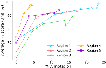
Effect of AL Cycles. We study how the EvaNet performance as measured by the average F1 score (i.e., average of the flood and dry F1 scores) improves with the AL cycles. Figure 5 shows the results, where the x-axis corresponds to the percentage of pixels annotated so far at the end of an AL cycle, and the curve for each region has 5 data points corresponding to 5 AL cycles on the region. We can see that both the percentage of annotated pixels and the average F1 score improve with more AL cycles, and the average F1 score can reach a high value in just 5 cycles. Also, since each pixel click may cover different number of pixels via elevation-guided BFS, the percentage of increased annotated pixels varies with the cycles and regions. Other than R4 where the improvement seems to converge, the other regions show a clear performance improving trend so running more cycles is likely to further boost the performance.
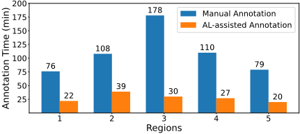
Effect of AL in Speeding up Annotation. We show the total time taken by manual annotation (with elevation-guided BFS) and AL-assisted annotation (with ALFA) for all test regions in Figure 6. The time reported here is the median time obtained from the user study. We can see that AL assistance significantly speeds up the annotation. We also consider another baseline where users use AL-assisted annotation for 2 cycles and then fix EvaNet mistakes manually. Without loss of generality, the results on R1 and R5 are presented in Table 4, where we can see that to reach a similar level of average F1 score, using AL throughout the annotation process can reduce time from over 40 minutes to around 20 minutes.
| Region | Method | Time (min) | Avg F1 score |
|---|---|---|---|
| R1 | AL Only AL + Manual | 22 | 98.93 |
| 46 | 98.95 | ||
| R5 | AL Only AL + Manual | 20 45 | 93.86 92.66 |
Table 4: ALFA for 5 cycles (AL Only) v.s. ALFA for 2 cycles followed by manually fixing EvaNet prediction errors (AL + Manual).
5 Conclusion
We presented ALFA, an active learning framework for flood annotation on earth imagery. ALFA integrates prediction confidence, view consistency, temporal consistency and tree score to calculate the uncertainty scores of individual pixels, which are aggregated in the unit of superpixels to recommend the most uncertain (hence informative) ones by the underlying EvaNet flood segmentation model for user annotation by elevation-guided BFS. ALFA also expands EvaNet's supervised elevation-guided loss function with two unsupervised loss terms for view consistency and temporal consistency, respectively, to improve retraining performance. Extensive experiments show that all our techniques are beneficial and ALFA can obtain high-quality annotation for flood mapping in a much short time than manual annotation.
Acknowledgements
The authors at Indiana University Bloomington were supported by DOE ECRP Award DE-SC0025228, NSF OAC2414474, NSF OAC-2414185, the Radiance Technologies Innovation Bowl grand prize awarded as the competition winner in 2023, and 2024-2025 Luddy Faculty Fellow Award from Indiana University Bloomington. The research of Sidharth Kumar and Steve Petruzza were funded by NSF SHF2401274, NSF SHF-2221812, and NSF PPoSS Planning Award 2217036 and Large Award 2316157.
@inproceedings{ijcai2025p1057,
  title     = {Faster Annotation for Elevation-Guided Flood Extent Mapping by Consistency-Enhanced Active Learning},
  author    = {Adhikari, Saugat and Yan, Da and Wang, Tianyang and Dyken, Landon and Kumar, Sidharth and Yuan, Lyuheng and Ahmad, Akhlaque and Han, Jiao and Zhou, Yang and Petruzza, Steve},
  booktitle = {Proceedings of the Thirty-Fourth International Joint Conference on
               Artificial Intelligence, {IJCAI-25}},
  publisher = {International Joint Conferences on Artificial Intelligence Organization},
  editor    = {James Kwok},
  pages     = {9511--9519},
  year      = {2025},
  month     = {8},
  note      = {AI and Social Good},
  doi       = {10.24963/ijcai.2025/1057},
  url       = {https://doi.org/10.24963/ijcai.2025/1057},
}
TY - CPAPER TI - Faster Annotation for Elevation-Guided Flood Extent Mapping by Consistency-Enhanced Active Learning AU - Adhikari, Saugat AU - Yan, Da AU - Wang, Tianyang AU - Dyken, Landon AU - Kumar, Sidharth AU - Yuan, Lyuheng AU - Ahmad, Akhlaque AU - Han, Jiao AU - Zhou, Yang AU - Petruzza, Steve T2 - Proceedings of the Thirty-Fourth International Joint Conference on Artificial Intelligence, IJCAI-25 PB - International Joint Conferences on Artificial Intelligence Organization PY - 2025 SP - 9511 EP - 9519 DO - 10.24963/ijcai.2025/1057 UR - https://doi.org/10.24963/ijcai.2025/1057 ER -Copied
Machine-readable versions of this paper, for tools and AI agents:





