
Hazard Function Guided Agent-Based Models: A Case Study of Return Migration from Poland to Ukraine
Proceedings of the Thirty-Fourth International Joint Conference on Artificial Intelligence. AI and Social Good. Pages 9818-9826.
https://doi.org/10.24963/ijcai.2025/1091
Keywords
- Multidisciplinary Topics and Applications: General
- Agent-based and Multi-agent Systems: General
Abstract
The Russian invasion of Ukraine in February 2022 has led to the largest forced migration crisis in Europe since World War II, with millions displaced both internally and internationally. Among the displaced, approximately 4.2 million individuals have returned, highlighting the significance of return migration as a critical phase in the migration continuum. Existing studies on return migration are limited in scope, relying on survey-based approaches that suffer from demographic bias, lack of validation against ground truth, and inability to account for uncertainty. We propose a novel computational framework for modeling the return of conflict-induced migrants, using agent-based models (ABMs) and their surrogates. These models are grounded in hazard functions and account for sociopolitical contexts. Our proposed ABMs outperform baseline methods in estimating return migration from Poland to Ukraine by at least 42% and by as much as 57% in terms of normalized root mean squared error (NRMSE). Further, to illustrate the utility of such models for policymakers, we conduct two case studies that estimate the duration of displacement and characterize the demographic breakdown among the returnees.
- [ACLED, 2010] ACLED. Introducing ACLED-Armed Con- flict Location and Event Data. Journal of Peace Research, 47(5):651-660, 2010.
- [Adhikari and Hansen, 2014] Prakash Adhikari and Wendy L Hansen. Reversing the flood of forced displacement: Shedding light on important determinants of return migration. https://digitalrepository.unm.edu/ nsc research/93/, 2014. Link
- [Ajzen, 1991] Icek Ajzen. The theory of planned behavior. Organizational behavior and human decision processes, 50(2):179-211, 1991.
- [Alrababah et al., 2023] Ala Alrababah, Daniel Masterson, et al. The dynamics of refugee return: Syrian refugees and their migration intentions. British Journal of Political Science, 53(4):1108-1131, 2023. [Associated Press, 2024] Associated Press. Israel-hezbollah ceasefire: Refugees return home to lebanon, 2024. Ac- cessed: 2025-02-08.
- [Auld et al., 2011] Joshua Auld, Taha Hossein Rashidi, et al. Dynamic activity generation model using competing hazard formulation. Transportation research record, 2254(1):28-35, 2011.
- [Azzarri and Carletto, 2009] Carlo Azzarri and Calogero Carletto. Modelling migration dynamics in albania: a haz- ard function approach. Southeast European and Black Sea Studies, 9(4):407-433, 2009.
- [Banerjee, 1992] Abhijit V Banerjee. A simple model of herd behavior. The quarterly journal of economics, 107(3):797-817, 1992.
- [Battistella, 2018] Graziano Battistella. Return migration: A conceptual and policy framework, 2018. Accessed: 2025- 02-08.
- [Billari et al., 2007] Francesco C Billari, Alexia Prskawetz, Belinda Aparicio Diaz, and Thomas Fent. The "wedding- ring" an agent-based marriage model based on social in- teraction. Demographic research, 17:59-82, 2007.
- [Biondo et al., 2012] Alessio Emanuele Biondo, Alessandro Pluchino, and Andrea Rapisarda. Return migration af- ter brain drain: A simulation approach. arXiv preprint arXiv:1206.4280, 2012.
- [Cassarino, 2008] Jean-Pierre Cassarino. Conditions of modern return migrants-Editorial introduction. Interna- tional Journal on Multicultural Societies, 10(2):95-105, 2008.
- [Chakraborty and Gupta, 2015] Subrata Chakraborty and Rameshwar D Gupta. Exponentiated geometric distri- bution: another generalization of geometric distribution. Communications in Statistics-Theory and Methods, 44(6):1143-1157, 2015.
- [Cox and Oakes, 1984] D.R. Cox and D. Oakes. Analysis of Survival Data. Chapman and Hall, New York, NY, 1984.
- [Cox, 1959] D. R. Cox. The analysis of exponentially dis- tributed life-time with two types of failures. Journal of Royal Statistical Society, 21B:411-421, 1959.
- [Cox, 1972] D. R. Cox. Regression models and life-tables. Journal of Royal Statistical Society, 26B:186-220, 1972.
- [Frazier, 2018] Peter I Frazier. A tutorial on bayesian opti- mization. arXiv preprint arXiv:1807.02811, 2018.
- [Granovetter, 1978] M. Granovetter. Threshold models of collective behavior. The American Journal of Sociology, 83(6):1420-1443, 1978.
- [Hancock et al., 2022] Matthew Hancock, Nafisa Halim, et al. Effect of peer influence and looting concerns on evacuation behavior during natural disasters. In Proc. of COMPLEX NETWORKS, 2022.
- [IOM, 2022] IOM. Ukraine internal displacement report: General population survey round 3, April 2022.
- [IOM, 2024] IOM. IOM:Displacement Tracking Matrix. https://dtm.iom.int/ukraine, 2024. Link
- [Kleinbaum and Klein, 2012] David G. Kleinbaum and Mitchel Klein. Survival Analysis -A Self-Learning Text. Springer, Heidelberg, Germany, 2012.
- [Kleinberg, 2000] Jon Kleinberg. The small-world phe- nomenon: An algorithmic perspective. In Proceedings of the thirty-second annual ACM symposium on Theory of computing, pages 163-170, 2000.
- [Lee and Horvitz, 2017] Dae Lee and Eric Horvitz. Predict- ing mortality of intensive care patients via learning about hazard. In Proc. of AAAI, volume 31, 2017.
- [Liu et al., 2017] Shenghua Liu, Houdong Zheng, Huawei Shen, Xueqi Cheng, and Xiangwen Liao. Learning concise representations of users' influences through online behav- iors. In IJCAI, pages 2351-2357, 2017. IJCAI
- [Maidanik, 2024] Iryna Maidanik. The forced migration from Ukraine after the full scale Russian invasion: Dy- namics and decision making drivers. European Societies, 26(2):469-480, 2024.
- [Mehrab et al., 2022] Zakaria Mehrab, Aniruddha Adiga, Madhav V Marathe, Srinivasan Venkatramanan, and Samarth Swarup. Evaluating the utility of high-resolution proximity metrics in predicting the spread of covid-19. ACM TSAS, 8(4):1-51, 2022.
- [Mehrab et al., 2024a] Zakaria Mehrab, Logan Stundal, et al. An agent-based framework to study forced migra- tion: A case study of ukraine. PNAS nexus, 3(3), 2024.
- [Mehrab et al., 2024b] Zakaria Mehrab, Logan Stundal, et al. Network agency: An agent-based model of forced migration from Ukraine. In Proc. of AAMAS, 2024.
- [Mehrab et al., 2025] Zakaria Mehrab, S.S. Ravi, et al. Hazard Function Guided Agent-Based Models: A Case Study of Return Migration from Poland to Ukraine. github.com/dmehrab06/ukr migration return/ blob/main/IJCAI 2025 Ukraine Return-Online.pdf, 2025. BII Technical Report: #2025-7. Link
- [Migration Observatory, 2011] Migration Observatory. De- mographic objectives in migration policy-making, 2011. Accessed: 2025-02-08.
- [Miller, 1981] Rupert G. Miller. Survival Analysis. John Wi- ley and Sons, New York, NY, 1981.
- [Mortveit et al., 2020] Henning. S Mortveit, Abhijin Adiga, et al. Synthetic Populations and Interaction Networks for the U.S., 2020. NSSAC Technical Report: #2019-025.
- [Pandey et al., 2023] Abhishek Pandey, Chad R Wells, et al. Disease burden among Ukrainians forcibly displaced by the 2022 Russian invasion. PNAS, 120(8), 2023.
- [Portal, 2022] Poland's Data Portal. Statistical data on the situation on the border with Ukraine. https://dane.gov.pl/ en/dataset/2705, 2022. Link
- [Qiu and others, 2022] Zirou Qiu et al. Understanding the coevolution of mask wearing and epidemics: A network perspective. PNAS, 119(26), 2022.
- [Rizzuto et al., 2017] Debora Rizzuto, René JF Melis, Sara Angleman, Chengxuan Qiu, and Alessandra Marengoni. Effect of chronic diseases and multimorbidity on survival and functioning in elderly adults. Journal of the American Geriatrics Society, 65(5):1056-1060, 2017.
- [S ¸ahin-Mencütek, 2024] Zeynep S ¸ahin-Mencütek. Concep- tual complexity about return migration of refugees/asylum seekers. Journal of Asian and African Studies, 59(7):2125-2138, 2024.
- [Saikia and Barman, 2017] Rinku Saikia and Manash Pratim Barman. A review on accelerated failure time models. Int J Stat Syst, 12(2):311-322, 2017.
- [Sohst et al., 2024] Ravenna Sohst, Tino Tirado, et al. Ex- ploring Refugees' Intentions to Return to Ukraine: Data Insights and Policy Responses. Migration Policy Insti- tute Europe and International Organization for Migration, Brussels and Geneva, 2024.
- [Sologoub, 2024] I. Sologoub. Return or stay? what factors impact the decisions of ukrainian refugees. VoxUkraine, 2024. [Studien, 2024] Forum Transregionale Studien. Why Ukrainians return: Motivations of return migration and its implications. https://trafo.hypotheses.org/53767, 2024. Link
- [Suresh et al., 2022] Krithika Suresh, Cameron Severn, and Debashis Ghosh. Survival prediction models: an intro- duction to discrete-time modeling. BMC medical research methodology, 22(1):207, 2022.
- [Toth-Bos et al., 2019] Agnes Toth-Bos, Barbara Wisse, and Klara Farago. Goal pursuit during the three stages of the migration process. International Journal of Intercultural Relations, 73:25-42, 2019.
- [UNHCR, 2023] UNHCR. Lives on Hold: Intentions and Perspectives of Refugees from Ukraine #3. https://data. unhcr.org/en/documents/details/99072, 2023. [UNHCR, 2024] UNHCR. Ukraine Refugee Situation. https://data.unhcr.org/en/situations/ukraine, 2024. [Ac- cessed December 30, 2024]. Link
- [Valente, 1996] Thomas W Valente. Social network thresh- olds in the diffusion of innovations. Social networks, 18(1):69-89, 1996.
- [van Tubergen et al., 2024] Frank van Tubergen, Gusta G Wachter, Yuliya Kosyakova, and Irena Kogan. Return in- tentions among Ukrainian refugees in Europe: A cross- national study. International Migration, 62(5), 2024.
- [Van Wijk and Simonsson, 2022] Rob C Van Wijk and Ul- rika SH Simonsson. Finding the right hazard function for time-to-event modeling: A tutorial and shiny applica- tion. CPT: Pharmacometrics & Systems Pharmacology, 11(8):991-1001, 2022.
- [World Bank, 2025] World Bank. Forced displacement, 2025. Accessed: 2025-02-08.
- [Wu et al., 2020] Sean L Wu, Andrew J Dolgert, Joseph A Lewnard, John M Marshall, and David L Smith. Princi- pled simulation of agent-based models in epidemiology. bioRxiv, pages 2020-12, 2020.
- [Wycoff et al., 2024] Nathan Wycoff, Lisa O Singh, Ali Arab, Katharine M Donato, and Helge Marahrens. The digital trail of ukraine's 2022 refugee exodus. Journal of Computational Social Science, 7(2):2147-2193, 2024.
- [Zetter, 2021] Roger Zetter. Refugees and their return home: Unsettling matters. Journal of Refugee Studies, 34(1):7- 22, 2021.
- [Zhou et al., 2021] Zhengyang Zhou, Yang Wang, Xike Xie, Lei Qiao, and Yuantao Li. Stuanet: Understanding un- certainty in spatiotemporal collective human mobility. In Proceedings of the Web Conference 2021, 2021.
References were extracted automatically from the PDF and may contain errors.
Full text extracted automatically from the PDF; figures, tables and equations may differ. The PDF is the version of record.
1 Introduction
The Russian invasion of Ukraine that began on February 24, 2022, has caused, among other things, the largest forced migration in Europe since the end of World War II [UNHCR, 2023]. As of August 2024, around 3.7M people have been reported to be internally displaced in various parts of Ukraine [IOM, 2024]. Around 6.8M people have been displaced as refugees, among which around 6.2M have taken shelter in various European countries [UNHCR, 2024]. According to the 2025 Humanitarian Needs and Response Plan, 12.7M people are estimated to be in need of multidimensional humanitarian assistance. One such dimension considers potential migrants who have already returned or who are seeking to return to Ukraine once the situation deescalates. The return migration to Ukraine began as early as April 2022. With the out-migration from Ukraine seemingly halted, return migration is the most prominent dimension that needs addressing at present.
Reports suggest that around 4.2M people have returned to Ukraine as of October 2024 [IOM, 2024]. Even though return migration is identified to be among the highest of priorities among the multi-dimensional top-down management issues surrounding international migration [Cassarino, 2008], there is a paucity of systematic literature surrounding return migration [Adhikari and Hansen, 2014; S¸ahin-Menc¨utek, 2024; Zetter, 2021; Toth-Bos et al., 2019]. In fact, available studies attempting to tackle return migration in the context of the conflict in Ukraine have relied on survey-based approaches [van Tubergen et al., 2024; Maidanik, 2024; Studien, 2024]. While potentially useful in identifying key factors driving return migration, three limitations raise concerns regarding the applicability of these survey-based approaches in the long run. First, these surveys are conducted with a subsample of the population, which can make these studies demographically biased. Second, models fitted from these survey responses are not validated against any ground truth observations, making their validity questionable. Third, models developed from these studies are not probabilistic, making them unable to account for the uncertainty associated with return migration, which is inherent in spatiotemporal human mobility [Zhou et al., 2021]. Thus, a computational tool that can overcome these limitations is imperative.
Contributions: To address the above limitations, we assembled a multidisciplinary team consisting of computer scientists and political scientists. By integrating AI-driven modeling and political science insights, our work makes the following contributions to address one dimension of the pressing societal challenge of forced displacement.
- First, Using the concept of hazard functions we propose three agent-based models (ABMs) to study return migration from a conflict-induced country by considering relevant contexts (e.g., social and political), with each ABM adding more contextual layers than the previous. We also propose surrogates to these ABMs that generate aggregated summary reports with lower computational expense. To the best of our knowledge, this is the first work that computationally models conflict-induced return migration without relying on survey-based approaches.
- Second, we evaluate our models against baselines and show their superiority in modeling the first wave of return migration from Poland to Ukraine, which lasted roughly until the end of July 2022. We also perform additional experiments to quantify the uncertainties in the model.
- Third, we conduct two case studies that underscore the utility of these models in generating policy-relevant information. The first case study involves finding the mean length of displacement. Validated against ground truth estimates from subsidiary reports, this study shows the accuracy of the emergent behavior of the ABM. The second case study, which analyzes the demographic patterns of returnees using the fast surrogate models, shows the efficacy of our model in ensuring fair resource allocation based on requirements.
2 RelatedWork
Return Migration: An early work [Biondo et al., 2012] that employed a computational approach to model return migration in the context of voluntary migration, assumed that each migrant has two associated social networks, one at home and another abroad. Using a single-agent perspective, they calculated utility at home and abroad as functions of the networks and decaying expectation, and when the utility abroad becomes less than the utility at home, they assumed that the migrant would return. Since the work was done in the context of voluntary migration and used a single-agent perspective, it is not directly applicable to our case. A more recent work [Alrababah et al., 2023] attempted to model return intentions of Syrian refugees based on survey responses of around 3000 refugees living in Lebanon. They identified safety at home and network effects to be the key factors behind return migration and commented that the effect of host countries do not play a significant role during short-term migration. A recent work [van Tubergen et al., 2024] studied return migration in the context of the Ukraine war by collecting survey responses from 18,000 Ukrainian refugees. They attempted to model return migration considering three perspectives: (a) contextual (e.g., economic, social attachment), (b) source country (e.g., security) and (c) cross country (e.g., language). Although done in the context of conflict-induced forced migration, these two studies are based on surveys, which are often time consuming. Furthermore, both works have acknowledged the respondent group to be demographically biased, which may fail to paint a general picture.
Hazard Function: Although hazard functions have been used extensively in areas such as biometrics and industrial engineering to examine life-expectancy and product failures [Lee and Horvitz, 2017; Rizzuto et al., 2017; Saikia and Barman, 2017], researchers have also applied them in other contexts. For example, Liu et al. [2017] applied hazard function to study influence of one user over another in social networks. Auld et al. [2011] developed a competing hazard model based on the Weibull hazard function and used it to simulate the daily activities of individuals. Azzarri et al. [2009] developed a duration model based on the loglogistic hazard to understand the factors behind migration and return of Albanian migrants, based on surveys. However, the method was developed in the context of voluntary migration and the temporal resolution was yearly, making it infeasible to study short-term conflict-induced migration. Finally, hazard functions have also been used in conjunction with ABMs in various domains. For example, Wu et al. [2020] used ABM simulation to infer the hazard of transmission and that of recovery. Billari et al. [2007] uses an ABM and a hazard function to study the influence of an agent's age and social pressure on the likelihood of the agent getting married. These examples illustrate applicability of ABMs in conjunction with hazard functions to model various social issues.
3 Methodology
3.1 Overview
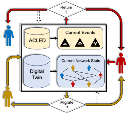
The concepts of hazard and survival functions lie at the core of our modeling. While existing literature attempts to quantify return intention by considering different combinations of factors based on survey responses, we start with the basic assumption that every migrant wants to return eventually. As we point out in this section, this latent intention can be accommodated in the simplest of our modeling approaches to the very complex ones. First, we discuss these models under the hood of the ABM framework, with the assumption that the time of migration of each agent is known, along with other properties. Subsequently, we discuss learnable surrogates of the ABMs which can be leveraged to generate important results with less computational expense.
3.2 Hazard and Survival Functions
Hazard and survival functions were conceptualized and further developed by Cox [1959; 1972]. We briefly review these concepts to make our paper self-contained. Additional information can be found in several textbooks (e.g., [Cox and Oakes, 1984; Kleinbaum and Klein, 2012; Miller, 1981]).
Hazard and survival functions are defined for a random variable T with an underlying probability distribution function (PDF) p(T = t) and a cumulative distribution function (CDF) F(T ≤ t) that gives the probability that an event has occurred by time t. The survival function S(t) is defined as the complement of the CDF. Thus, S(t) = 1 - F(t) = ∫ ∞ t p(x)dx, which gives the probability that the event of interest has not occurred by time t.
The hazard function h(t) is often defined in conjunction with the survival function. Considering the event of interest as a failure, h(t) is interpreted as the instantaneous rate of failure given that the failure has not occurred by time t. Mathematically, h(t) is defined by h(t) = p(t) S(t) = - ∂ ∂t logS(t). It follows that S(t) = exp (- ∫ t 0 h(u)du).
3.3 ProblemFormulation
Let A be the set of agents and X be the set of conflict-induced regions. Each agent a ∈ A has the following attributes. First, their migration time T M a , the time at which agent a migrates to a different country. For agents a who never migrate, we set T m a =∞. Second, their origin xa ∈ X. Additionally, let GA(A, EA) be the network formed by the agent set A where EA corresponds to the agent pair who may exert peer influence over one another. Let Na be the set of agents who are the neighbors of agent a induced by the edges EA. We assume that the edge set EA does not change over time.
Let ha(t > T m a ) denote the hazard rate of an agent at time t that represents instantaneous rate of the agent failing to stay migrated (i.e., returning to xa). While recurring movements are possible, we assume that agents only leave their countries of migration when their goal is return migration. Applying the formula for S(t) in the discrete-time scenario, the probability Sa(t + 1) that the agent will stay migrated at time t + 1 given that it has remained a migrant up to time t, can be written as Sa(t +1) = exp (- ∑tt′=0 ha(t′ )). By doing a Bernoulli sampling based on Sa(t) (where Bern(p) indicates that the Bernoulli trial leads to success with probability p), we can estimate return state of an agent at time t. Formally, let ra(t) denote the state whether an agent has returned by time t or not. Then, ra(t) ∼ Bern(Sa(t)) tells us the return state of agent a at time t (if the agent has not already returned). Thus, modeling the hazard function ha(t) will allow us to control the return dynamics in various ways. Subsequent sections describe how we employ various strategies to progressively refine the hazard function by employing various societal factors that play a key role in conflict-induced migration scenarios. Across all the models ha(t ≤ T m a ) = 0, which constrains agents from returning before migration. Thus, from here on, ha(t) corresponds to ha(t > T m a ).
3.4 ABMof ReturnMigration
Model 1: Basic Hazard (BASE)
Motivation: In the context of forced migration, it is well established that the general intention of displaced individuals is to eventually return to their place of origin [Zetter, 2021].
Therefore, the decision to return can be effectively seen as a time-to-event problem, where the "event" is the act of returning. The hazard function is often used for survival analysis in discrete-time simulation [Suresh et al., 2022]. Thus, it is a natural choice for modeling return migration dynamics.
Formulation: Various forms of hazard functions are used in the literature. A comprehensive list of these various forms, along with their mathematical properties and corresponding survival functions has been described in [Van Wijk and Simonsson, 2022]. Our initial model uses the simplest of these forms where we consider the hazard rate to be constant for all agents at all times. Thus, the ABM is characterized by:
It indicates that at any time t > T m a , agent a has a constant value h of baseline hazard rate that controls their likelihood of returning if they have not already returned by that time. It can be shown that, if the hazard rate is constant, the underlying probability distribution for the time to return can be expressed as a geometric distribution [Chakraborty and Gupta, 2015]. Thus, P (ra(t) = 1) = h × (1 - h)t-T m a , ∀a, ∀t.
Agent Dynamics: Thus, the Basic Hazard Guided ABM works as follows. Initializing the baseline hazard rate h, at every time step t, all the agents a with T m a < t and ra(t-1) = 0 calculate Sa(t) (probability of not returning) based on the baseline hazard h. Then, ra(t) is sampled from Sa(t).
A more nuanced analysis can be conducted by classifying the agents into groups and assigning each group a separate hazard rate. While we explore this in a case study, our goal is to provide the foundation for adding more layers of complexity starting from the simplest of assumptions. Therefore, while acknowledging the possibility of agent class-based hazard rates, we refrain from doing so in our initial evaluations.
Model 2: Conflict Context Influenced Hazard (CL)
Motivation: Having established the basic ABM for modeling return migration, we next consider what other contexts to incorporate in calculating the hazard rate and how to incorporate them. Several survey reports conducted on Ukrainian migrants to identify key factors behind their intention to return can help us in this regard. One report published by IOM [Sohst et al., 2024] indicates that improved security situation in origin community/Ukraine is the primary motive behind Ukrainian refugees' return in the short term. In another, safety was marked as the primary factor for return by more than 45% of the participants [Sologoub, 2024].
Formulation: We incorporate conflict context for modeling return migration dynamics into the ABM as follows. Let, Za ⊆ X denote the regions observed by agent a. Let c(z, t) denote the conflict context 1 of region z at time t. We use this conflict context to modify the baseline hazard rate as follows.
Here, L is a lag parameter that controls the time of the latest conflict context. Since migration decisions involve planning and travel time [Wycoff et al., 2024], choosing such parameter is important for temporal mapping of a migrant from intending to return to being recorded as a returnee at the border. The window parameter W is used to reduce the effect of noise present in the data recording conflict context [Mehrab et al., 2022]. Finally, K is a normalizing constant so that the rightside term of the multiplication is bounded between 0 and 1. In the evaluation section, we describe how these are configured. From Equation (2), we can see that when the conflict context is high, the baseline hazard will be scaled down, indicating that the likelihood of return will decrease and vice-versa.
1 Conflict context is a scalar quantity to measure the intensity of conflict in a region at a particular time. More details are in Section 4.
Agent Dynamics: Thus, the Conflict Context Influenced Hazard Guided ABM works as follows. At every discrete-time step t, all the agents a with T m a < t and ra(t - 1) = 0 look at the conflict contexts of each region z ∈ Za from time t - L -W to t - L and incorporate it to scale the baseline hazard h following Equation (2). This scaled hazard is used to calculate the return probability of each agent.
Researchers have used other forms of hazard functions (e.g., Weibull) to include additional covariates [Auld et al., 2011]. However, these covariates are added in the exponent term while the baseline hazard rate is kept as separate. Since conflict context is significant to return dynamics, we choose this functional form to let it affect the baseline hazard. Moreover, the other forms of hazard functions have additional parameters. Since this study aims at developing the simplest possible model with a minimal set of parameters, we refrain from using functional forms that introduce additional parameters and complexities.
Model 3: Conflict and Peer influenced Hazard (CL P)
Motivation: According to many social and behavioral theories (e.g., theory of planned behavior [Ajzen, 1991], herd behavior [Banerjee, 1992]), peer influence is a key factor behind driving one's decisions. It has also been established that both conflict events and peer influence are important in driving migration decision-making [Mehrab et al., 2024b]. Following this, in our final model, we incorporate peer influence along with conflict context. We do so using the threshold model, a well-known model used for capturing peer influence [Valente, 1996; Granovetter, 1978]. Traditionally threshold model is used in the context of peer influence by having agents go through state transition when the number of neighbors with a particular state exceeds some threshold [Hancock et al., 2022; Qiu and others, 2022]. Since we are modeling the return state with hazard function, we use the threshold model instead to have the agents transition using different hazard functions.
Formulation: Let, qa(t) = ∑a′∈Na ra′(t) be the number of neighbors of a who have returned by time t. We express ha(t) in the form of a piecewise hazard function as follows.
Here, τa (0 ≤ τa ≤ 1) is the fractional active threshold parameter required to influence agent a. Since considering different thresholds across agents is difficult, we consider a simpler model where each agent has the same fractional active threshold parameter (i.e., ∀a ∈ A, τa = τ). While we do not impose any constraint here, ideally one can expect hℓ to be larger than hs, since when more people are returning it should drive a neighboring agent more likely to return.
Agent Dynamics: Thus, the Conflict Context and Peer Influenced Hazard Guided ABM works as follows. At every time step t, all the agents a with T m a < t and ra(t - 1) = 0 look at the fraction of their neighbors who have migrated and returned. If the fraction is larger (smaller) than τ, they choose a baseline hazard of hℓ (hs). Then, they look at the conflict contexts of each region z ∈ Za from time t - L - W to t -L and incorporate it to scale the baseline hazard and subsequently calculate the return probability using it.
It can be seen that we have progressively added layers to our model to incorporate contexts of different dimensions, making the models progressively more powerful in capturing return migration dynamics. However, as this has two additional parameters (a different baseline hazard and the threshold), it will be computationally more expensive to calibrate.
3.5 Surrogate Models of ReturnMigration
In this section, we propose some surrogates to the ABMs operating in the aggregated population space rather than the individual agent space. While we lose some granularity by doing so, we significantly reduce the computational cost.
The problem formulation for return migration in the aggregated population space is as follows. Let M = ⟨m(1),m(2), ...,m(T)⟩ be the temporal estimates of migrants, where m(t) is the number of migrants at time t. We define R to be the T ×T return matrix, where ri,j is defined as the number of returnees at time i among those who migrated at time j. Thus, by definition, when i ≤ j, ri,j = 0. Our goal is to find the values ri,j, ∀i, j : i > j. We will refer to these as the non-trivial entries of the Rmatrix. In the remainder of this subsection, we describe three surrogates corresponding to the three proposed ABMs; each description shows how the non-trial values of R are computed.
Surrogate to the BASE model
Let h be the constant hazard rate defined as the parameter of BASE. Let Qi,j denote the number of remaining migrants at the time i from time j who survive (i.e., do not return), calculated by Qi,j = m(j) - ∑k<i rk,j . Thus, the surrogate to BASE computes the non-trivial entries ri,j as follows.
Surrogate to the C L Model
Similar to how the problem space in the aggregated population space, the surrogate also assumes conflict context at a global level. Let htc be the conflict-influenced hazard expressed as htc = h × (1 - 1K ∑x∈X ∑Wt′=0 c(x, t - t′ - L)), where W,K,L have similar meanings as described for C L. Thus, the non-trivial entries ri,j can be calculated as follows.
Surrogate to the C L P model
Since C L P considers peer influence at the local neighborhood level of agents, an exact formulation of this peer influence is difficult for the surrogate working at aggregated population space. We approximate the peer influence as follows. Let, ˜ r(t) = ∑tt′=1 ∑t′ j=1 ri,j be the total number of people who have returned by time t. Let htcp be the conflict and peer influenced hazard expressed as follows.
where N is the total number of agents. This essentially is a peer influence considered at the overall population level instead of the local neighborhood level. Using this, this surrogate calculates non-trivial ri,j as follows.
Here, the exponent term contains the conflict and peerinfluenced hazard term hicp which is defined above. It can be seen that while these surrogate models can generate aggregated level outputs, they cannot generate detailed individual agent level behavior. However, since the outputs of surrogate models can be generated with great computational efficiency, if they are similar to the results of ABM, they can be used as components of beneficial software tools for policymakers.
3.6 Model Calibration
In order to find a parameter configuration (e.g., hazard rate, threshold parameter) that best fits the model, we define a loss function that combines the capability of the model to capture the scale and trend of the observed return estimate and apply a black-box optimization technique, namely Bayesian optimization, to optimize this loss function. Bayesian optimization is applied when the parameter space has a small dimension (typically < 20), the objective function is computationally extensive and its gradient is non-trivial to evaluate ([Frazier, 2018]).
Let Rθ = ⟨rθ(1), rθ(2), ..., rθ(T)⟩ be daily return estimates provided by our models (ABM or surrogate) parameterized by θ. Let, ˜R = ⟨˜ r(1), ˜ r(2), ..., ˜ r(T)⟩ be the observed number of returnees which we want to calibrate our model. We define the following loss function.
The first term calculates the root mean squared error (RMSE) between the model estimate and the ground truth estimate whereas the second term calculates the Pearson correlation coefficient (PCC) between the model estimate and the observed estimate. Here, λe and λc are weight coefficient hyperparameters. Our proposed loss can help the model avoid getting stuck in local minima in terms of just the traditional RMSE loss. We present a justification for this claim and perform experiments to validate our claim in the online supplementary material [Mehrab et al., 2025]
| Baseline | NACRPS | NRMSE | PCC | |||
|---|---|---|---|---|---|---|
| L21 | N/A | 0.223 | 0.569 | |||
| L30 | N/A | 0.213 | 0.617 | |||
| L40 | N/A | 0.211 | 0.628 | |||
| L45 | N/A | 0.207 | 0.647 | |||
| NACRPS | NRMSE | PCC | ||||
| Ours | ABM | S-ABM | ABM | S-ABM | ABM | S-ABM |
| BASE C 21 | 0.067 | 0.062 | 0.12 | 0.131 | 0.95 | 0.92 |
| 0.059 | 0.060 | 0.112 | 0.135 | 0.93 | 0.91 | |
| C 21 P | 0.057 | 0.062 | 0.106 | 0.126 | 0.93 | 0.91 |
| C 30 P | 0.051 | 0.083 | 0.089 | 0.102 | 0.95 | 0.93 |
| C 35 P | 0.052 | 0.051 | 0.094 | 0.128 | 0.96 | 0.94 |
| C 40 P | 0.056 | 0.054 | 0.107 | 0.169 | 0.95 | 0.89 |
4 Evaluation
The following subsection provides an overview of the configurations of our experiments and the subsequent subsections describe the results and case studies. All evaluation and studies involve the case of the return migrants from Poland to Ukraine during the early period of the Russian invasion of Ukraine. While we cannot comprehensively evaluate the generalizability of the model due to inadequacy of ground truth pertaining to diverse scenario, we emphasize that our model can be applied in other conflict scenarios as well.
4.1 Experimental Setup
Datasets: We parse the conflict events of Ukraine during the Feb-Aug 2022 period from ACLED [2010]. For the agent data, we use the synthetic household data described in [Mortveit et al., 2020]. We collect the synthetic households of Ukraine and the associated synthetic individuals. These households represent the agents in our model. Finally, we obtain the border-crossing data from Polish border guards [Portal, 2022] and use the number of Ukrainians crossing a Poland-Ukraine border between February 24, 2022 and August 01, 2022 as the ground truth.
Building Block Models: Since our problem formulation requires knowing the migration time of the agents to estimate their return time (Figure 1), we first apply the ABMTPB model [Mehrab et al., 2024a] to assign each migrant a refugee or internally displaced (IDP) status. Then, we apply the method proposed in [Pandey et al., 2023] to place each refugee in one of the six neighboring countries of Ukraine and apply our methodology on the refugees placed in Poland. To account for the uncertainties associated with these models, we run 100 realizations of ABM-TPB model to create a Digital Library (DL) of simulations (see supplementary material [Mehrab et al., 2025] for details) by using Latin Hypercube Sampling (LHC) over the parameter spaces for ABMTPB. From the DL, we select the 30 best performing simulations. Then, we run our models for return migration over each of these simulations 30 times.
Hyperparameters: We create the agent network GA using Kleinberg's Small World Model (KSW) [2000] using the methods and parameters described in [Mehrab et al., 2024b]. The same network is also used for the ABM-TPB model. Across all the C L and C L P models, we use a constant window parameter W = 7 days and the lag parameter L ∈ {21, 30, 35, 40} days. To reduce the number of possible covariate combinations, we also set Za = X, ∀a ∈ A for our ABM models. Future research can explore how limiting the scope of observation to different radii of neighboring regions can change the outcome of the model and how this can be done across agents of various demographic groups. Finally, we use daily total fatalities from ACLED as the conflict context to our ABMs and their surrogates and K is chosen to be the maximum value among all conflict contexts.
Metrics: We first evaluate Normalized Root Mean Squared Error (NRMSE), to measure accuracy of the model estimation. The second metric is Normalized Average Continuous Ranked Probability Score (NACRPS), used to quantify how well the model can account for uncertainty in its estimation. Finally, we also evaluate the Pearson Correlation Coefficient (PCC) to quantify how well the model can capture the trend in the observed data. These metrics are described in detail in the online supplementary material [Mehrab et al., 2025].
Baseline: As baselines for our models, we create some vanilla linear regression models LD , D ∈ {20, 30, 40, 45}. Here, D represents the number of days of historical conflict contexts each model uses as features. For these models, we consider both the number of events and the fatalities of events as conflict context. Note that these models are not probabilistic in nature; so, they cannot account for uncertainties.
(b) Surrogate of C30 P
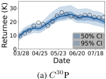
Figure 2: Best Performing ABM and Surrogates for estimating return migrants from Poland to Ukraine. Circles represent ground truth data. Visualizations corresponding to other models of Table 1 can be found in the online Supplement. 50% (95%) CI corresponds to the 50% (95%) confidence interval of the model estimate.
4.2 Experimental Validation
Table 1 summarizes the performance of our proposed models against the baseline methods. We describe our main findings in the next two subsections. For a more comprehensive set of experiment results, see the online supplementary material [Mehrab et al., 2025].
Error and Correlation: The best ABM (C 30 P) has a median NRMSE of 0.089, an improvement of around 57% compared to the best-performing regressor (L45 , with an NRMSE of 0.207). Even the simplest ABM (BASE) has a 42% improvement in NRMSE compared to L45 . The surrogates also outperform the baseline methods. The best-performing surrogate (surrogate of C 30 P) has a median NRMSE of 0.102, a 51% improvement over L45 . Further, our proposed models capture the trend of the return migration better than baseline methods, with PCC constantly being higher than 0.9. These results underscore the capability of the proposed hazard-based models to capture the scale and trend of the return migration accurately. Notably, C L P models always seem to perform better than BASE or C L, thus bringing out the importance of considering different layers of sociopolitical contexts in capturing return dynamics. We elaborate on this through an ablation study (see Supplementary material [Mehrab et al., 2025]).
Surrogate vs ABM: The proposed surrogate models are able to produce estimates comparable to their ABM counterparts. We take the C 30 P as an example, which has the best performance in terms of NRMSE. Its surrogate has an NRMSE of 0.102, which is worse only by 14.6% compared to the NRMSE of its ABM counterpart. However, the surrogate model takes around three seconds to generate the return estimate whereas the ABM takes close to 10 minutes for one instance to execute. Such a significant improvement in computation time may compensate for the penalty in accuracy. However, it must be noted that the more sub-optimal the ABM gets, the performance of its surrogate gets progressively worse. For example, the performance drop in NRSME of the surrogate for C 35 P is almost 36.1% (0.128 vs 0.094) and for C 40 P is around 57%. This behavior also underscores the importance of choosing a good lag parameter. Effect of the lag parameter is further discussed in the online Supplementary material [Mehrab et al., 2025].
4.3 Uncertainty Quantification
It is important to quantify the uncertainty associated with a probabilistic model designed for generating return migration estimates. To do so, we analyze the NACRPS of the models tabulated in Table 1. First, we notice that adding layers of complexity to BASE decreases NACRPS, suggesting improvement of both point forecasts and probabilistic forecasts. Second, the C L P ABMs with lower NRMSE have low NACRPS as well; thus, these models not only have reasonable point prediction accuracy, but the uncertainty associated with probabilistic return estimation is also accounted for more effectively. Third, adding layers of complexity to the surrogate models do not necessarily improve NACRPS. As example, when conflict context is introduced with the BASE, the NACRPS slightly improves with a decline in NRMSE. But, when peer influence is added, the NACRPS declines as NRMSE improves. Thus, there is a tradeoff between accuracy and uncertainty across these surrogate models. If we compare the C 30 P surrogate with its ABM counterpart in Figure 2, we realize that the poor NACRPS of the surrogate is due to high uncertainty interval (shaded region) at the later period (Figure 2b), which does not happen for the ABM (Figure 2a). In the ABM, since peer influence comes from the local neighborhood of each agent, the threshold is unlikely to be met by all agents at once. For the surrogates, peer influence is calculated by looking at the entire population. Thus, the transition occurs for everybody simultaneously. Across multiple simulations, uncertainty propagated by this sharp transition is observed intensely, leading to higher NACRPS values.
5 Case Studies
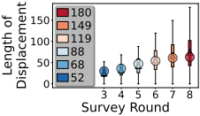
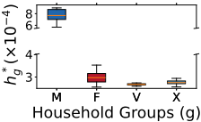
Figure 3: Two case Studies conducted using our proposed models
5.1 Return Time Estimation
For our first case study, we aim to understand an aspect of utmost importance to policymakers. The question we want to address is the following. What is the expected length of displacement before someone conducts return migration? An answer to this question helps policymakers to decide whether the migrants require long-term integration programs or shortterm emergency responses [World Bank, 2025]. It can also help policymakers plan for advocating a ceasefire on various frontlines, given migrants displaced from vicinities return after a certain period [Associated Press, 2024].
To answer this question, we calculate the length of stay across agents at different periods of the Ukraine war using the output from the C 30 P ABM. Figure 3a shows distribution of the length of displacement, along with the reported mean length of displacement provided in the IOM general survey reports [IOM, 2022]. We can see that the reported mean length agrees well with the model estimates. Moreover, the increase in the length of displacement before return with the progression of the war is correctly estimated by our model. This signifies that our proposed hazard-guided ABM is appropriate for time-to-return modeling as this emergent behavior matches qualitative observation and captures overall return migration dynamics.
5.2 Demographic Pattern of Returnees
Our second case study aims to estimate the demographic composition of returning migrants. Since ground truth containing demographic details is not available regarding return migrants, such estimates can help policymakers in tailoring targeted reintegration initiatives [Battistella, 2018] or allocating social/medical services based on the psychological needs of specific demographic groups [Migration Observatory, 2011]. Here, the question we want to address is: What is the likelihood of return for migrants from different demographic groups? Fitting hazard rate parameters across various demographic groups can answer this question.
| Group | Household Description | Migrant ratio (%) |
|---|---|---|
| M | Adult males only | 1.47±0.41 |
| F | Adult females only | 6.07±0.23 |
| V | Elderly (and/or) children | 71.64±0.34 |
| X | Adult males and females | 20.81±0.16 |
Therefore, we modify the surrogate of BASE as follows. We first categorize each household into one of the four groups outlined in Table 2. Then, we initialize hg, ∀g ∈ {M, F, V,X} and the surrogate model produces return estimates for the groups individually. The aggregation of return estimates of all groups is calibrated to match the total return estimates Once calibrated, the hazard rates of individual groups in Figure 3b reveal interesting emergent properties.
First, we notice that the adult male-only households have a high hazard rate compared to other groups. This indicates their high propensity to return to Ukraine, which can be attributed to the mandate requiring adult males to participate in the war. Second, we observe that households with vulnerable groups (i.e., elderly, children) are the least likely to return. This implies that the threat of security is greatest among families with children and elderly. Third, we observe that female-only households have hazard rates similar to the vulnerable groups compared to the male-only households, again indicating their greater concern for security compared to adult males. Consequently, females without partners are slightly more likely to return than females with male partners, which corroborates with prior findings [Sologoub, 2024], indicating the possibility of having a partner alongside to be more motivating to settle in a new place. Finally, there is less variance in hazard rate across the V group, compared to the other groups. Since the largest portion of migrants is comprised of this group, a slight variation from the calibrated hazard rate may cause a large deviation from the ground truth. Overall, the ability to produce demographically detailed estimates underscores the usefulness of the model in building decisionsupport tools for policymakers.
6 Concluding Remarks
We developed novel agent-based models (ABMs) for return migration, experimentally evaluated these models and conducted case studies using these models to demonstrate their usefulness in generating policy-relevant information. Our models can be seamlessly incorporated to work with prior computational models that generate outflow of Ukrainian migrants and subsequently place them in one of the neighboring countries. Therefore, our work provides the path to develop the first end-to-end ABM of forced migration that is jointly able to capture these heterogeneous migration dynamics. Future work can explore the return dynamics of internally displaced people and consequently, address the dynamics of recurring migration.
Ethical Statement
The work reported in this paper proposes agent-based models for studying several aspects of returning migrants during conflicts. Such models are useful in developing software tools that will be beneficial to policymakers. The paper presents simulation-based evaluations of the models using a synthetic dataset discussed in one of the cited references and other public domain datasets.
Acknowledgements
This work was supported in part by NSF grant #2053013, DTRA contract HDTRA1-19-D-0007, NSF grant OAC1916805 , NSF Expeditions in Computing grant CCF1918656, UVA Strategic Investment Fund award number SIF160, and the Strategic Investment Fund Award to the UVA's Humanitarian Collaborative. We would also like to thank the reviewers for their insightful feedbacks.
@inproceedings{ijcai2025p1091,
  title     = {Hazard Function Guided Agent-Based Models: A Case Study of Return Migration from Poland to Ukraine},
  author    = {Mehrab, Zakaria and Ravi, S. S. and Stundal, Logan and Swarup, Samarth and Venkatramanan, Srini and Lewis, Bryan and Mortveit, Henning and Leblang, David and Marathe, Madhav V.},
  booktitle = {Proceedings of the Thirty-Fourth International Joint Conference on
               Artificial Intelligence, {IJCAI-25}},
  publisher = {International Joint Conferences on Artificial Intelligence Organization},
  editor    = {James Kwok},
  pages     = {9818--9826},
  year      = {2025},
  month     = {8},
  note      = {AI and Social Good},
  doi       = {10.24963/ijcai.2025/1091},
  url       = {https://doi.org/10.24963/ijcai.2025/1091},
}
TY - CPAPER TI - Hazard Function Guided Agent-Based Models: A Case Study of Return Migration from Poland to Ukraine AU - Mehrab, Zakaria AU - Ravi, S. S. AU - Stundal, Logan AU - Swarup, Samarth AU - Venkatramanan, Srini AU - Lewis, Bryan AU - Mortveit, Henning AU - Leblang, David AU - Marathe, Madhav V. T2 - Proceedings of the Thirty-Fourth International Joint Conference on Artificial Intelligence, IJCAI-25 PB - International Joint Conferences on Artificial Intelligence Organization PY - 2025 SP - 9818 EP - 9826 DO - 10.24963/ijcai.2025/1091 UR - https://doi.org/10.24963/ijcai.2025/1091 ER -Copied
Machine-readable versions of this paper, for tools and AI agents:





