
Scalable Graph Classification via Random Walk Fingerprints (Extended Abstract)
Proceedings of the Thirty-Fourth International Joint Conference on Artificial Intelligence. Sister Conferences Best Papers. Pages 10912-10915.
https://doi.org/10.24963/ijcai.2025/1215
Keywords
- Sister Conferences Best Papers: Data Mining
Abstract
We design a lightweight structural feature extraction technique for graph classification. It leverages node subsets and connection strength reflected by random-walk-based heuristics, presenting a scalable, unsupervised, and easily interpretable alternative. We provide theoretical insights into our technical design and establish a relation between the extracted structural features and the graph spectrum. We show our method achieves high levels of computational efficiency while maintaining robust classification accuracy.
- [Berlingerio et al., 2013] Michele Berlingerio, Danai Koutra, Tina Eliassi-Rad, and Christos Faloutsos. Net- work similarity via multiple social theories. In ASONAM, pages 1439-1440, 2013.
- [Borgwardt and Kriegel, 2005] Karsten M Borgwardt and Hans-Peter Kriegel. Shortest-path kernels on graphs. In IEEE ICDM, 2005.
- [Cai and Wang, 2018] Chen Cai and Yusu Wang. A simple yet effective baseline for non-attribute graph classification. ICLR workshops, 2018.
- [Dong et al., 2019] Kun Dong, Austin R Benson, and David Bindel. Network density of states. In ACM SIGKDD, pages 1152-1161, 2019.
- [Errica et al., 2020] Federico Errica, Marco Podda, Davide Bacciu, and Alessio Micheli. A fair comparison of graph neural networks for graph classification. In ICLR, 2020.
- [Feragen et al., 2013] Aasa Feragen, Niklas Kasenburg, Jens Petersen, Marleen de Bruijne, and Karsten Borgwardt. Scalable kernels for graphs with continuous attributes. NeurIPS, 26, 2013.
- [Fosdick et al., 2018] Bailey K Fosdick, Daniel B Lar- remore, Joel Nishimura, and Johan Ugander. Configuring random graph models with fixed degree sequences. SIAM Review, pages 315-355, 2018.
- [Hamilton et al., 2017] Will Hamilton, Zhitao Ying, and Jure Leskovec. Inductive representation learning on large graphs. NeurIPS, 2017.
- [Hido and Kashima, 2009] Shohei Hido and Hisashi Kashima. A linear-time graph kernel. In IEEE ICDM, pages 179-188, 2009.
- [Huang et al., 2021] Leo Huang, Andrew J Graven, and David Bindel. Density of states graph kernels. In SDM, pages 289-297. SIAM, 2021.
- [Kipf and Welling, 2017] Thomas N. Kipf and Max Welling. Semi-supervised classification with graph convolutional networks. In ICLR, 2017.
- [Kojaku and Masuda, 2018] Sadamori Kojaku and Naoki Masuda. Core-periphery structure requires something else in the network. New Journal of physics, 20(4):043012, 2018.
- [Li et al., 2024] Peiyan Li, Honglian Wang, and Christian Böhm. Scalable graph classification via random walk fin- gerprints. In 2024 IEEE International Conference on Data Mining (ICDM), pages 231-240. IEEE, 2024.
- [Pan et al., 2022] Liming Pan, Cheng Shi, and Ivan Dok- manić. Neural link prediction with walk pooling. In ICLR, 2022.
- [Rozemberczki and Sarkar, 2020] Benedek Rozemberczki and Rik Sarkar. Characteristic functions on graphs: Birds of a feather, from statistical descriptors to parametric models. In Proceedings of the 29th ACM international conference on information & knowledge management, pages 1325-1334, 2020.
- [Rozemberczki et al., 2020] Benedek Rozemberczki, Oliver Kiss, and Rik Sarkar. Karate Club: An API Oriented Open-source Python Framework for Unsupervised Learn- ing on Graphs. In CIKM, page 3125-3132, 2020.
- [Sawlani et al., 2021] Saurabh Sawlani, Lingxiao Zhao, and Leman Akoglu. Fast attributed graph embedding via den- sity of states. In IEEE ICDM, pages 559-568, 2021.
- [Shervashidze et al., 2011] Nino Shervashidze, Pascal Schweitzer, Erik Jan Van Leeuwen, Kurt Mehlhorn, and Karsten M Borgwardt. Weisfeiler-lehman graph kernels. JMLR, 12(9), 2011.
- [Tsitsulin et al., 2018] Anton Tsitsulin, Davide Mottin, Panagiotis Karras, Alexander Bronstein, and Emmanuel Müller. Netlsd: hearing the shape of a graph. In ACM SIGKDD, pages 2347-2356, 2018.
- [Verma and Zhang, 2017] Saurabh Verma and Zhi-Li Zhang. Hunt for the unique, stable, sparse and fast feature learning on graphs. NeurIPS, 2017.
- [Vishwanathan et al., 2010] S Vichy N Vishwanathan, Nicol N Schraudolph, Risi Kondor, and Karsten M Borgwardt. Graph kernels. JMLR, 11:1201-1242, 2010.
- [Xu et al., 2019] Keyulu Xu, Weihua Hu, Jure Leskovec, and Stefanie Jegelka. How powerful are graph neural net- works? In ICLR, 2019.
References were extracted automatically from the PDF and may contain errors.
Full text extracted automatically from the PDF; figures, tables and equations may differ. The PDF is the version of record.
1 Introduction
We address the problem of graph classification. Similar to classifying text or image data, comparing graphs is fundamental to building a classifier. This task, known as graph similarity learning, is challenging due to the inherent variability in both the size and structure of the graphs.
Targeting graph similarity, the past decade has witnessed the success of graph kernels [Shervashidze et al., 2011; Borgwardt and Kriegel, 2005] and graph representation learning [Kipf and Welling, 2017; Tsitsulin et al., 2018]. The former compares substructures, while the latter utilizes supervised graph neural networks, or uses unsupervised embedding approaches paired with classifiers. Despite their success, scalability remains a critical issue. This is due to the increasing size of real-world graphs and the large volume of graph datasets, as both the scale of each graph and the number of graphs can be substantial. To address the scalability challenge, we introduce RandomWalk Fingerprints (RWF), an unsupervised structural feature extraction technique that can incorporate node attributes. The computational complexity of RWF is bounded by O(Nτc(mn + pn2 )), where N is the number of graphs; n and m are the number of nodes and edges per graph; τc is the maximum walk steps; and p is the dimension of node features. In the worst-case scenario where m = n2 , RWF exhibits a cubic time complexity regarding n. However, the typical sparsity of real-world graphs (m≪n2 ) generally ensures more manageable computational demands.
1 This is an extended abstract of a paper first published in the IEEE ICDM conference [Li et al., 2024].
2 Method
At its core, RWF quantifies intra- and inter-subset connection strengths among node subsets with distinct structural roles. By focusing on these role-based subsets, RWF enables soft alignment between structurally heterogeneous graphs, enabling meaningful comparisons. Based on these node subsets, heuristics like loop and walk, reflecting the connection strength, are used to construct the feature vector. Additionally, RWF can easily incorporate node features. After feature extraction, we use a basic classifier like SVM to get the classification results.
Structural-Role-based Vertex Partitioning
We divide the nodes of each graph into distinct subsets, thereby facilitating alignment among the node subsets across disparate graphs. This essential step enables us to identify local graph patterns, thus enhancing the representation power of our method. Given a graph G, we partition its nodes into k subsets, i.e., V = V1 ∪ · · · ∪ Vk, where each subset contains nodes that share the same structural role, and k is the number of predefined roles. In order to obtain size-invariant representations of graphs, the parameter k should be consistent for all graphs.
- Degree Heuristic. Degree is an essential statistic of nodes. High-degree nodes tend to be cores in the local central regions, while low-degree nodes often occupy peripheral positions. Hence, node degree serves as a naive indicator of the structural roles of nodes. Initially, we count the node degrees. We then sort the nodes by their degrees and divide the node set into k subsets, each containing |V |/k nodes.
- Core-Periphery Heuristic. This heuristic is based on the assumption that the arrangement of a graph includes densely connected core nodes and sparsely connected peripheral nodes. We utilize KM-config [Kojaku and Masuda, 2018] to identify core and peripheral nodes. It leverages the configuration model [Fosdick et al., 2018] as the null model to generate a target graph with idealized core-periphery pairs. Then, it maximizes the similarity between the target and source graphs through appropriate node labeling. Notably, KM-config can detect multiple core-periphery pairs, and it has a linear time complexity with respect to the number of edges.
Structural Feature Extraction
With the node partitions of each graph determined, subsequently, we show how to extract features based on the graph G and its node partitions (V1, V2, · · · , Vk). In the simplest form, we quantify the connection strength within and between the subsets of nodes based on the relational matrix T and its powers. The relational matrix T can be defined by the transition matrix Tp = D-1A, or the symmetric normalized adjacency matrix T = D- 12 AD- 12 , where D denotes the diagonal degree matrix and A denotes the adjacency matrix. Each entry of Tp and T quantifies a kind of connection strength between two nodes. In this paper, we select T since symmetric normalization enables computational efficiency. We introduce the following features.
Here, loopτVi represents the average strength of all τ-loops of nodes in Vi. walkτVi represents the average strength of all τ-walks that start and end at nodes within Vi. walkτVi→Vj denotes the average strength of all τ-walks traversing from Vi to Vj. In a nutshell, the three features measure the connection strength within and between node subsets.
Incorporation of Node Attributes
In addition to the structural features, our method is designed to incorporate node features. Accordingly, we define the following two matrices:
where P ∈ Rp×p and Q ∈ Rp×p are symmetric matrices encapsulating the interactions of node features within the node set Vi. Here, diag(TτVi ) and TτVi serve as kernels to modulate the influence of node features, while 1 |Vi| and 1 |Vi|2 are used to balance the numerical values. We further compute the row average of P and Q, producing two vectors xlτVi ∈ Rp and xwτVi ∈ Rp , which represent the aggregated features of the subset Vi at scale τ. This procedure yields a rich feature vector for the node subset that combines sub-structural and node-feature-based information.
3 Feature Interpretation
We demonstrate the connections between the extracted features and the graph spectrum, providing insight into the use of local feature extraction and a limited walking length.
Connections to Graph Spectrum
We factorize T as follows:
where the columns of U ∈ Rn×n are eigenvectors of T, and Λ is the diagonal matrix whose diagonal elements are the corresponding eigenvalues, denoted by {Λ1, · · · ,Λn}. Let UVi ∈ R|Vi|×n be the rows of U that corresponds to Vi, specifically, we use the node indices of Vi to extract a subset of rows of U to form UVi .
Let B = UTVi UVi , which is a symmetric n×n matrix, and {α1, α2, · · · , αn} are the corresponding diagonal entries. Let β = {β1, · · · , βn} ∈ R1×n and γ = {γ1, · · · , γn} ∈ R1×n be the row vector with the sum over each column of UVi and UVj , respectively. We have:
The above calculations establish the relationship between the three feature sets and the spectrum of Tτ , i.e., the three features represent the weighted aggregation of the eigenvalues of Tτ . Thus, the extracted features could be conceptualized as ensembles that capture the essence of the full eigenvalue spectrum of the graph. This connection may elucidate the efficacy of the extracted features, as several studies (e.g., [Tsitsulin et al., 2018; Dong et al., 2019; Sawlani et al., 2021]) have demonstrated the effectiveness of graph spectrum in graph classification tasks.
Why Use Local Feature Extraction?
Consider A as the adjacency matrix of an undirected graph. We alter an arbitrary edge euv by adjusting its weight, and the updated adjacency matrix becomes ˆA. After applying symmetric normalization to A and ˆA, we get T and ˆT, which denote the initial and modified transition matrices, respectively. We use d(x, y) to represent the shortest path distance between two nodes x and y. For the perturbed edge uv, we introduce a distance function d(w) = min{d(w, u), d(w, v)}, which measures the minimum distance from any node w to either node in the pair u or v. We give the following theorem derived from [Pan et al., 2022]. We have a different setting regarding T but the proof is the same.
Based on the above theorem, it is easy to understand that under structural perturbation, the change in T propagates outward from the perturbed nodes to their increasingly distant neighbors as the number of walk steps increases. If we omit the vertex partitioning process and only use loopτV and walkτV as features, we can still distinguish A and ˆA. But with vertex partitioning and the three features defined, it is possible to detect where the perturbation occurs, as node subsets act as local sensors. Therefore, vertex partitioning may enhance the distinguishing power of the defined features.
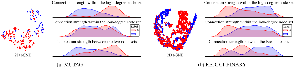
Fig. 1 shows the results of RWF on two graph datasets. Recall that the underlying assumption behind RWF is that graphs from different classes exhibit distinct local connectivity patterns. These patterns are reflected by node subsets that assume different structural roles. In the simplest form, we categorize the nodes of each graph into two subsets: high-degree and low-degree. Then we fix the maximum walk step τc to 6 and calculate {loopτVhigh , walkτVhigh }τc τ=1 , {loopτVlow , walkτVlow }τc τ=1 and {walkVhigh→Vlow }τc τ=1 . This division gives rise to three distinct feature domains: the connectivity strength within high-degree nodes, within lowdegree nodes, and between high-degree and low-degree nodes. As illustrated in Fig. 1, RWF features demonstrate strong discriminatory capabilities. Moreover, we can observe distinctions between the distributions of different classes, even when considering a single domain of RWF features independently.
Why Limit Walk Steps?
We explain why we use a limited number of steps as controlled by τc. Due to the symmetric normalization, the eigenvalues of T are bounded within the interval [-1, 1]. Based on the above calculations, it is evident that the three features can be expressed as weighted aggregations of the eigenvalues of Tτ , like f(τ) = ∑nt=1 δtΛτt , where the vector δ = {δ1, · · · , δn} ∈ R1×n contains some constant values. Without loss of generality, we assume the eigenvalues are sorted in descending order, with Λ1 and Λn representing the maximum and minimum eigenvalues, respectively. The maximum eigenvalue Λ1 = 1. The minimum eigenvalue Λn = -1 if and only if the corresponding graph is bipartite; otherwise, Λn lies in the range of (-1, 0]. For simplicity, we assume Λn follows the latter case, as bipartite graphs are special, and we consider general cases here. When τ becomes large:
The above calculation reveals that f(τ) ≈ δ1 when τ is large, and δ1 is a constant. This suggests that larger τc does not contribute additional structural information. In practice, we set τc to a value typically not exceeding 10 to ensure efficiency while capturing meaningful graph structure.
4 Experimental Evaluation
We evaluate our method against the following techniques:
- Unsupervised graph embedding algorithms: NetLSD [Tsitsulin et al., 2018], NetSimile [Berlingerio et al., 2013], FGSD [Verma and Zhang, 2017], A-DOGE [Sawlani et al., 2021], LDP [Cai and Wang, 2018] and FEATHER [Rozemberczki and Sarkar, 2020].
| DEE | RED-12K | GIT | TWI | |
|---|---|---|---|---|
| NetLSD | 56.1 | 38.5 | 64.6 | 68.6 |
| A-DOGE | 55.6 | 47.8 | 67.0 | 69.5 |
| FGSD | 56.2 | 33.2 | 60.7 | 64.2 |
| NetSimile | 55.6 | 47.3 | 68.8 | 70.5 |
| FEATHER | 55.7 | 47.2 | 69.0 | 70.0 |
| LDP | 55.6 | 46.8 | 67.2 | 68.5 |
| NH | 56.0 | ‡ | 60.2 | ‡ |
| WL | 55.6 | 39.5 | 62.6 | ‡ |
| DOSGK | 55.7 | ‡ | 66.3 | ‡ |
| GCN | 56.8 | 45.9 | 61.3 | 69.0 |
| GraphSAGE | 56.8 | 42.2 | 53.7 | 61.4 |
| GIN | 56.9 | 47.3 | 61.4 | 68.7 |
| RWF-CP | 57.1 | 43.6 | 66.7 | 69.6 |
| RWF-CP-feature | 56.6 | 46.2 | 70.4 | 69.1 |
| RWF-D | 56.5 | 44.8 | 68.1 | 71.3 |
| RWF-D-feature | 55.9 | 48.1 | 70.4 | 71.4 |
- Graph kernels: NH [Hido and Kashima, 2009], WL [Shervashidze et al., 2011], and DOSGK [Huang et al., 2021].
- Graph neural networks: GCN [Kipf and Welling, 2017], GIN [Xu et al., 2019], and GraphSAGE [Hamilton et al., 2017].
Due to brevity, we only show the results on four large datasets. The reader can find all the experiments in [Li et al., 2024].
The graph classification results on Deezer ego nets (DEE), REDDIT-MULTI-12K (RED-12K), Github stargazers (GIT), and Twitch egos (TWI), are reported in Table 1. RWFs achieve the best results in general.
5 Conclusion
In this paper, we proposed RWF, a scalable, interpretable, unsupervised feature extraction approach for graph classification. RWF learns a subset-based representation of graphs, central to which is the structural-role-based vertex partitioning scheme. This technique enables soft alignments across diverse graphs and thus facilitates the learning of local structures. Specifically, RWF extracts three features, measuring the connection strengths within and between node subsets. Additionally, a highlight of RWF is its flexibility in incorporating node attributes, making it a comprehensive tool for feature extraction. Our experimental analysis confirms the effectiveness and efficiency of RWF, illustrating its potential as a powerful approach to graph classification.
@inproceedings{ijcai2025p1215,
  title     = {Scalable Graph Classification via Random Walk Fingerprints (Extended Abstract)},
  author    = {Li, Peiyan and Wang, Honglian and Böhm, Christian},
  booktitle = {Proceedings of the Thirty-Fourth International Joint Conference on
               Artificial Intelligence, {IJCAI-25}},
  publisher = {International Joint Conferences on Artificial Intelligence Organization},
  editor    = {James Kwok},
  pages     = {10912--10915},
  year      = {2025},
  month     = {8},
  note      = {Sister Conferences Best Papers},
  doi       = {10.24963/ijcai.2025/1215},
  url       = {https://doi.org/10.24963/ijcai.2025/1215},
}
TY - CPAPER TI - Scalable Graph Classification via Random Walk Fingerprints (Extended Abstract) AU - Li, Peiyan AU - Wang, Honglian AU - Böhm, Christian T2 - Proceedings of the Thirty-Fourth International Joint Conference on Artificial Intelligence, IJCAI-25 PB - International Joint Conferences on Artificial Intelligence Organization PY - 2025 SP - 10912 EP - 10915 DO - 10.24963/ijcai.2025/1215 UR - https://doi.org/10.24963/ijcai.2025/1215 ER -Copied
Machine-readable versions of this paper, for tools and AI agents:





