Bimodal Depth-First Search for Scalable GAC for AllDifferent

1 Introduction

Constraint programming (CP) [Rossi et al., 2006] enables the declaration of decision variables with potential values (domains) and constraints. A CP solver finds assignments that meet these requirements. CP uses synergy between propagation and search, where each component reinforces the other. Search systematically explores the solution space, assigning values to variables and verifying constraints. When a conflict arises, backtracking reverts decisions. Propagation narrows the search space, preventing exhaustive enumeration. It analyses variables and constraints to identify and remove inconsistent values. Filtering algorithms implement this propagation. Because eliminating all inconsistent values is NP-Hard, one must make a trade-off between propagation and search.

Global constraints (GC) with stronger filtering. GC is a key concept in CP, enabling efficient propagation by considering the interactions between several variables. For example, the ALLDIFFERENT constraint [R´egin, 1994] ensures distinct values for variables in a set. Global constraints exploit problem structure to provide stronger filtering, often aiming for high levels of consistency, such as Generalised Arc Consistency (GAC) or Bound Consistency (BC). GAC prunes all inconsistent values from the constraint's scope. BC relaxes domains to intervals, enabling faster filtering but less pruning.

Graph-based filtering algorithms and their bottlenecks. Graph algorithms using Depth-First Search (DFS) are crucial for filtering GC. They are often applied to the Variable-Value Graph (VVG), a bipartite graph where one set of vertices represents variables and the other set corresponds to possible values. Edges link variables to their feasible values. For example, R´egin's algorithm is applied to the VVG and enforces GAC for ALLDIFFERENT. However, DFS becomes a bottleneck whenever the graph is dense, as it runs in Θ(n + m) time, where n and m are the numbers of vertices and edges.

Bimodal DFS as away to address theDFSbottleneck. To allow faster graph traversal, [Dahlhaus et al., 2002] proposed a minimum-sized 'partially complemented' (p-c) graph representation consisting of either storing the successors or the non-successors. Its size is n+ ˜mwhere ˜m is the sum, for each vertex v, of the minimum between the numbers of successors and non-successors of v. This representation allows some graph algorithms' runtime to depend on ˜m instead of m. In a CP context, the VVG may start out very dense then become sparse, or some subsets of vertices may have a few successors, while others many. Thus, algorithms with ˜m-dependent complexities are very appealing. However, the domain representations prevent these p-c algorithms from being used on the VVG. This motivated us to introduce bimodal DFS, which is inspired by the p-c DFS but leverages the ability of many solvers to (A1) efficiently iterate over a domain (the successors of a variable in the VVG) and (A2) efficiently check if a value is present (whether an edge belongs to the VVG).

Contributions. Our main contributions include:

1. A configurable bimodal DFS, whose worst-case time complexity is O(n + ˜m) under assumptions (A1)-(A2), as well as a bimodal Breadth-First Search (BFS) algorithm used for finding a matching in the VVG.
2. Bimodal BFS and DFS integrated into R´egin's GAC algorithm for ALLDIFFERENT. It outperforms state-ofthe-art GAC algorithms on large instances and comes close to the speed of the BC algorithm of [L´opez-Ortiz et al., 2003] in practice.

Paper organisation. Sect. 2 gives related work on efficient DFS and GAC algorithms for ALLDIDFFERENT and on the partially complemented representation of graphs. Sect. 3 gives our 1st contributions: bimodal BFS and DFS. It introduces the tracking list, a data structure used in bimodal DFS. Sect. 4 integrates these results in the GAC filtering of ALLDIFFERENT. Sect. 5 presents the conducted experiments. Some details are given in the technical appendix. 1

1 Technical appendix: https://hal.science/hal-05062193

2 RelatedWork

The Depth-First Search (DFS) algorithm is a fundamental algorithm used in many filtering algorithms. It handles constraints like ALLDIFFERENT, CIRCUIT [Lauri`ere, 1978; Kaya and Hooker, 2006], or SAME [Beldiceanu et al., 2006], where the computation of Strongly Connected Components (SCC) is potentially invoked an exponential number of times throughout the search, both on dense and on sparse graphs derived from variable domains.

Within CP, despite identifying DFS as a major bottleneck due to its need to traverse all graph edges, progress has only yielded constant speedup. For instance, for the GAC filtering algorithm of the ALLDDIFFERENT constraint [R´egin, 1994], these include optimising or dispensing with the DFSbased SCC algorithm [Gent et al., 2008; Zhang et al., 2018; Zhang et al., 2021; Zhen et al., 2023; Li et al., 2023] or utilising GPUs [Tardivo et al., 2023]. This has also prompted the use of incomplete filtering algorithms that prioritise BC over GAC [L´opez-Ortiz et al., 2003].

Partially Complemented Graphs. A number of studies in the literature have explored the potential for reducing the time complexity for constructing a BFS-forest and a DFS-forest of a graph by compressing its size significantly. Indeed, since the size of a forest is bounded by the number of vertices n, one would ideally like to construct it in O(n) time.

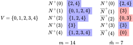
In particular, [Dahlhaus et al., 2002] introduced the Partially Complemented Representation (p-c representation) of a directed graph (digraph) D = (V,A), which consists, for every vertex v ∈ V , in either storing its successors N+(v) = {w ∈ V : (v,w) ∈ A} or its non-successors N+(v) = {w ∈ V : (v,w) /∈ A} (v is then said to be complemented). It is possible to obtain a minimum-sized p-c representation ˜D of D. Indeed, with n = |V | and d+(v) = |N+(v)|, for each v ∈ V : if d+(v) < n - d+(v) then N+(v) is stored, otherwise N+(v) is stored. Then, with ˜m = ∑v∈V min(d+(v ), n - d+(v )) and m = |A|, the size of the minimum-sized p-c representation ˜D is n+ ˜m. Also, ˜D is constructed in O(n+m) time with an adjacency list encoding of D. See Fig. 1.

It has been demonstrated that several graph algorithms [Dahlhaus et al., 2002; Lindzey, 2014; Joeris et al., 2017], including BFS and DFS, can be adapted to the p-c representation, resulting in a time complexity that depends on the size of ˜D rather than the size of the graph D itself. This is a very interesting property when | ˜D| ≪ |D|, which is the case, for example, when the graph is very dense.

3 Bimodal Algorithms for BFS and DFS

We propose CP-oriented variants of the classical BFS and DFS graph traversal algorithms, called Bi-BFS and Bi-DFS, based on the operations iteration and check. In a digraph D = (V, A) and for a vertex v ∈ V , the iteration operation allows one to iterate over the successors N+(v) of v, while the check operation determines whether a vertex is a successor of v. Their time complexities are denoted I(v) and C(v) respectively.

To illustrate these operations and their complexities, we take the example of the adjacency list (AL) and adjacency matrix (AM) graph representations. With AL, iterating over the successors of a given vertex v is done in O(d+(v)) time, and assessing the presence of a vertex in N+(v) is done in O(d+(v)) time too, so I(v) = O(d+(v)) and C(v) = O(d+(v)) for all v ∈ V . With AM, iterating over the successors of a given vertex v is done in O(n) time, and assessing the presence of a vertex in N+(v) is done in O(1) time, so I(v) = O(n) and C(v) = O(1) for all v ∈ V .

Graph representations in CP do not allow one to directly use the p-c algorithms, but they may offer efficient implementations for both iteration and check, as explained in the first paragraph of Sect. 4. That is why we design graph traversal algorithms based on these two operations. Our algorithms take a Boolean function f as additional input, defining the strategy for choosing between iteration or check for each vertex. This makes them configurable. We assume that f(v) is computed in constant time for all v ∈ V .

When looking for the unvisited successors of the currently explored vertex v, one can use iteration to iterate over the successors of v and explore the unvisited ones, or iterate over the unvisited vertices and use check to find the successors of v to explore. The worst-case time complexity of the bimodal BFS and DFS are stated in Theorems 1 and 2 and parametrised by f(v), I(v) and C(v), ∀v ∈ V . Under the assumptions of Corollaries 1 and 2, they achieve a O(n+ ˜m) time complexity like in the partially complemented approach, but without using the minimum-sized p-c representation.

Before presenting Bi-BFS and Bi-DFS, we briefly recall in Sect. 3.1 a doubly linked list that will represent the set of unvisited vertices. In Sect. 3.3, we define a new function for this list to enable Bi-DFS achieving the desired complexity.

3.1 Backtrackable Doubly Linked List

Knuth's dancing links technique [Knuth, 2000] allows for efficient reversal of doubly linked list operations. Thus, we call such list a backtrackable doubly linked list (bdll). Each node v points toward a predecessor v.pred and a successor v.succ in the list. The artificial node source has no predecessor, and the artificial node sink has no successor. The nodes form a chain from source to sink. The crux of the dancing links concept is the retention of the predecessor and successor of a deleted node. This ensures that reinserting the last removed node is done in constant time.

Definition 1 (Backtrackable Doubly Linked List Functions). We remind and define the elementary functions of the bdll:

• prev(v) returns the predecessor of v: return v.pred
• next(v) returns the successor of v: return v.succ

• hasNext(v) returns TRUE iff v is not at the end of the list: return v.succ ̸= sink
• remove(v) removes v from the list, assuming v is in the list and is neither source nor sink: v.pred.succ ← v.succ; v.succ.pred ← v.pred;
• reinsert(v) inserts v in the list, assuming v is the last removed node: v.pred.succ ← v; v.succ.pred ← v;
• present(v) returns TRUE iff v is in the list: return v.pred.succ = v

Note that each of these functions runs in O(1) time.

3.2 Bimodal Breadth-First Search

The BFS of [Dahlhaus et al., 2002] is an iterative algorithm that runs in O(n + ˜m) time once ˜D has been constructed. In contrast, our bimodal BFS algorithm (1) does not need to build ˜D, but uses D's iteration and check operations.

Using the bdll L to represent the set of unvisited vertices enables us to iterate efficiently over unvisited vertices and check in constant time whether a vertex has already been visited. We denote as d+ BFS(v) the number of outgoing arcs from v in the resulting BFS-forest.

Theorem 1. Bi-BFS goes through a BFS-forest of D and the time spent exploring a vertex v ∈ V is:

• O(I(v)) if f(v) = TRUE;
• O(C(v) × (n-d+(v) +d+ BFS(v))) if f(v) = FALSE.

Proof. If f(v) = FALSE, when iterating over the unvisited vertices during the exploration of v, these vertices are either successors of v forming the BFS-forest's arcs (v, w) (exactly d+ BFS(v)), or non-successors of v (at most n - d+(v)).

Corollary 1. If ∀v ∈ V , I(v)=O(d+(v)), C(v)=O(1) and f(v)= (d+(v) < n2 ), then Bi-BFS runs in O(n+ ˜m) time.

Proof. The BFS-forest is a forest, therefore ∑v∈V d+ BFS(v ) ≤ n. And then, by using the definition of ˜m and Theorem 1, we get the claimed complexity.

Algorithm 1 Bimodal BFS (Bi-BFS)

Require: A digraph D = (V, A) and a Boolean function f over V

Ensure: Explore a BFS-forest of D 1: L← V ; ▷ L is a bdll with the vertices in V 2: while L ̸= ∅ do EXPLOREBFS(L.next(L.source)); 3: procedure EXPLOREBFS(root) 4: Q←empty queue; 5: Q.enqueue(root); L.remove(root); 6: while queue Q is not empty do 7: v ← Q.dequeue(); 8: if f(v) then ▷ use iteration on N+(v) 9: for w ∈ N+(v) : L.present(w) do 10: Q.enqueue(w); L.remove(w); 11: else ▷ use check on N+(v) 12: w ← L.source; 13: while L.hasNext(w) do 14: w ← L.next(w); 15: if w ∈ N+(v) then 16: Q.enqueue(w); L.remove(w);

3.3 Bimodal Depth-First Search

While BFS was easy to adapt, DFS presents some difficulties. For partially complemented graphs, [Dahlhaus et al., 2002] proposed an iterative algorithm using a so-called complement stack, achieving a time complexity of O(n+ ˜m) once ˜D is constructed. [Joeris et al., 2017] presented a simpler recursive algorithm with the same time complexity, but requiring the lists of non-successors to be sorted in the same order. We propose a recursive algorithm that uses the operations iteration and check of D, without creating ˜D.

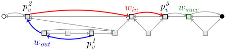
In the case of DFS, it is more difficult to efficiently iterate over the list L of unvisited vertices, since this list may change between two visits to the same vertex. To obtain the same complexity results as in Theorem 1, we avoid iterating several times over the same unvisited vertices for all visits to a given vertex v. To do this, we use a pointer pv that records the last position in L before finding a successor of v to explore. However, the position pointed by pv may be removed from L between two visits of v, which would force to iterate from the start of L at the next visit of v. To address this issue, we introduced in Definition 2 a new data structure called tracking list, which is a bdll with an extra function trackPrev. This function, illustrated in Figure 2, takes a node v as an argument, possibly removed from the list, and follows the prev pointers until it finds a node that currently belongs to the list.

Definition 2 (Tracking List). A tracking list is a bdll to which we add the following elementary function:

• trackPrev(v) returns the first node in the list from v by successively moving to the predecessor: track ← v;

while ¬present(track ) do track ← prev(track ); return track ;

Algorithm (2) provides the Bi-DFS procedure, which is based on iteration and check combined with the tracking list to explore a DFS-forest of D. Let d+ DFS(v) denote the number of outgoing arcs from v in the resulting DFS-forest.

Theorem 2. Bi-DFS goes through a DFS-forest of D, and the time spent exploring a vertex v ∈ V is:

• O(I(v)) if f(v) = TRUE;
• O(C(v) × (n-d+(v) +d+ DFS(v))) if f(v) = FALSE.

Proof. The proof outline is provided here; the complete proof is in Sect. 1 of the technical appendix. The main difficulty lies in proving that pv does not traverse too many nodes during all visits of v. Consider an iteration of the loop at line 9, which represents a single visit to the node v. In Bi-DFS we distinguish three positions for pv : (i) just before line 10 at

Algorithm 2 Bimodal DFS (Bi-DFS)

Require: A digraph D = (V, A) and a Boolean function f over V

Ensure: Explore a DFS-forest of D 1: L← V ; ▷ L is a tracking list with the vertices in V 2: while L ̸= ∅ do EXPLORE(L.next(L.source)); 3: procedure EXPLORE(v) 4: L.remove(v); 5: if f(v) then ▷ use iteration on N+(v) 6: for w ∈ N+(v) : L.present(w) do EXPLORE(w); 7: else ▷ use check on N+(v) 8: pv ← L.source; 9: while L.hasNext(pv ) do ① 10: pv ← L.trackPrev(pv ); ② 11: while L.hasNext(pv )∧L.next(pv ) /∈ N+(v) do 12: pv ← L.next(pv ); ③ 13: if L.hasNext(pv ) then EXPLORE(L.next(pv ));

①, denoted p 1 v ; (ii) just before lines 11-12 at ②, denoted p 2 v ; (iii) just after lines 11-12 at ③, denoted p 3 v .

We prove that (a) every node traversed by pv is a nonsuccessor of v, and that (b) every node traversed by pv is traversed at most once between p 1 v and p 2 v (e.g. wout in Fig. 3), and at most once between p 2 v and p 3 v (e.g. win in Fig. 3) over all visits of v. This leads to the given complexity.

Proof. TheDFS-forest is a forest so ∑v∈V d+ DFS(v) ≤ n. And then, by using the definition of ˜m and Theorem 2, we get the claimed complexity.

4 The Bimodal Approach for Filtering the ALLDIFFERENT Constraint

We extend the bimodal approach to filter the constraint ALLDIFFERENT. As R´egin [R´egin, 1994]'s GAC algorithm uses graph algorithms on the variable-value graph and a similar graph, we can rely on the domains of the variables rather than constructing these graphs directly. This allows us to take advantage of the domain operations for graph algorithms, including iteration and check on which the bimodal approach is based. Many domain representations offer efficient time complexities on these operations, such as successor vector [Van Hentenryck et al., 1992] and sparse set [de SaintMarcq et al., 2013], for which the iteration over the domain (iteration) is done in linear time in its size, and assessing the presence of a value (check) is done in constant time. This is what motivated the design of the bimodal approach.

The main theoretical contribution of this paper lies in the bimodal graph traversal algorithms, and, more specifically, in Bi-DFS presented in Sect. 3. Therefore, the pseudo-code for filtering ALLDIFFERENT with the bimodal approach is only presented in the technical appendix.

4.1 ALLDIFFERENT and R´egin's GACAlgorithm

The constraint ALLDIFFERENT on a set X of variables with their domains D = {D(x) : x ∈ X}, ensures that each variable in X has a different value. Based on the notion of variable-value graph and residual graph that we will introduce in Def. 3 and 4, an efficient GAC algorithm for ALLDIFFERENT was proposed by [R´egin, 1994].

Definition 3 (Variable-Value Graph, [Gent et al., 2008]). Let X be a set of variables and D their domains. Let V = ⋃x∈X D(x) be the set of possible values. The variablevalue graph is the bipartite graph G = (X ∪ V,E) with E = {(x, v) ∈ X ×V : v ∈ D(x)}.

Definition 4 (Residual Graph, [Gent et al., 2008]). Let X be a set of variables, D be their domains, V = ⋃x∈X D(x) and M be a maximum matching of the variable-value graph. The residual graph is the digraph G = (X ∪V ∪{t}, A) with t an artificially added vertex and A = {(x, v) ∈ (X × V )\M : v ∈ D(x)} ∪ {(v, x) ∈ V × X : (x, v) ∈ M} ∪ {(t, v) ∈ {t}×V : v ∈M} ∪ {(v, t) ∈ V ×{t} : v /∈M}.

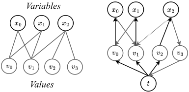
The algorithm prunes all variable-value pairs that cannot belong to a solution. It computes a Maximum Matching (MM) in the variable-value graph, and then filters out all pairs that do not belong to the same Strongly Connected Component (SCC) in the residual graph, as illustrated by Fig. 4.

We define r = |X|, d = |V | and m = ∑x∈X |D(x)|. We assume that r ≤ d, otherwise, the constraint is not met.

Maximum Bipartite Matching. There are many algorithms for finding a maximum matching in a bipartite graph, including the Hopcroft-Karp (HK) algorithm [Hopcroft and Karp, 1973], which runs in O(√rm) time, and the Kuhn algorithm, a subroutine of the Hungarian algorithm [Kuhn, 2004], similar to the Ford-Fulkerson algorithm [Leiserson et al., 1994], running in O(rm) time, but with better practical behaviour than HK [Setubal, 1993; Setubal, 1996].

[Gent et al., 2008; Zhen et al., 2023] uses Kuhn's algorithm, which is easy to implement and efficient. Given a current matching M in the graph, it performs a BFS from an unmatched vertex to find an augmenting path starting from it. If a matched vertex v is encountered during the BFS, it pursues the exploration from its partner M(v). The BFS stops when it finds an unmatched vertex, or when all vertices were explored. In the BFS tree, the path from the root to the encountered unmatched vertex is an augmenting path. It swaps edges on the augmenting path, increasing the matching size by 1. Repeating this process until all vertices are matched or no augmenting path is found produces a maximum matching.

Strongly Connected Components. To compute the SCC of the residual graph, R´egin uses Tarjan's algorithm [Tarjan, 1972], which runs in O(r +m) time. It performs a DFS on the graph's vertices, storing the pre-visit order for each vertex v as v.pre. It then calculates v.low, which is the most ancient vertex reachable from v in the pre-visit order. It uses a stack ST to store the visited vertices still unassigned to an SCC, and if a vertex is the root of an SCC (v.pre = v.low during the post-visit of v), then v and every vertex on top of it in ST are in the same SCC and therefore removed from ST .

Domain Filtering. To ensure GAC, arcs between SCCs not in the matching are pruned. When an SCC C is found, either its outgoing or incoming arcs can be pruned. We choose to prune the outgoing arcs, which come from variables in C and point to values outside C.

4.2 Our Bimodal Approach for ALLDIFFERENT

Using the domain representation, we directly run graph algorithms on the variable-value and residual graphs without explicitly building them. Thus, we only use the iteration and check operations of the domains and do not access the variables containing a given value. We adjust the definition of ˜m to the variable-value graph, which is bipartite: ˜m = ∑x∈X min(|D(x)|, d-|D(x)|). For the complexity results stated in this section, we suppose that I(x)=O(|D(x)|), C(x) = O(1), f(x) = (|D(x)| < d2 ) and that we can get |D(x)| in constant time for all x ∈ X.

Bimodal MM in the Variable-Value Graph

To find a maximum matching in the variable-value graph, we use Kuhn's algorithm, replacing the BFS with Bi-BFS. BiBFS starts at an unmatched variable, finding values to queue using either iteration or check on the variable's domain, based on the choice function f. When it encounters a value v, if v is matched then it continues the exploration from variable M(v), otherwise it stops the search. The list of unvisited vertices L contains values only, and no variables, because the values have at most one successor in the variablevalue graph: their matched variable. So, finding the unique successor of a value in the resulting BFS-tree is immediate.

By Corollary 1, this leads to an O(d+ ˜m) time complexity for each call to Bi-BFS. Thus, the overall time complexity for finding a maximum matching is O(k × (d + ˜m)), where k is the initial number of unmatched variables. Without using an incremental matching [R´egin, 1994], k should be replaced by r. See Sect. 2 of the technical appendix for further details.

Bimodal SCC of the Residual Graph

To compute the SCCs of the residual graph, we use Tarjan's algorithm, but modify it slightly to integrate Bi-DFS.

Bi-DFS is run from the matched values not yet visited, which is equivalent to starting the search from the artificial node t, whose pre-visit order is set to 0. A variable x is necessarily explored from its matched value M(x), so both are either in the same SCC or alone. For this reason, pre-visit orders and low points are only calculated for values, not for variables, and ST contains values only.

• When exploring a variable x with a small domain (f(v) = TRUE), we follow Tarjan's algorithm: for each value v in x's domain, if v is unvisited, we process it; if v is visited and in ST , then M(x).low gets the minimum between M(x).low and v.pre.
• If x has a large domain (f(v) = FALSE), we find the next unvisited value of x as in Bi-DFS and process it.

If no unvisited values remain in the second case, we look for the oldest visited value vanc of x that is still in ST. To do this, we iterate over ST from the bottom until we reach a value in D(x) or a value whose pre-visit order is greater than M(x).low, since the values in ST are sorted in ascending previsit order. M(x).low gets the minimum between M(x).low and vanc.pre. Observing this sole vertex vanc is sufficient for the algorithm to be correct, as noted in [Gent et al., 2008; Joeris et al., 2017].

Processing an unvisited value v involves (i) exploring M(v) if v is matched, and then setting M(x).low to the minimum of M(x).low and v.low, or (ii) v leads to the artificially added vertex t if v is unmatched, so M(x).low gets 0 and we continue the exploration from x.

The search for the oldest unassigned visited value vanc of a variable x is done in O(d - |D(x)|) time. And as with bimodal MM, the list of unvisited vertices L contains values only. Then to find the SCCs of the residual graph, this leads to a time complexity of O(d+ ˜m) by Corollary 2. See Sect. 3 of the technical appendix for further details.

Bimodal Domain Filtering

For an SCC C of the residual graph, we prune all variablevalue pairs (x, v) ∈ (X∩C×V ∩C : v ∈ D(x))\M (with C = V \C). This is done using the same method as the bimodal approach. Let x be a variable in C: if x has a small domain (i.e. f(x) = TRUE), iterate over D(x) and remove the values in C; if x has a large domain (i.e. f(x) = FALSE), iterate over the values in C and remove them from D(x).

A bdll serves as a representation of C. It is initialised with V . Each time an SCC C is processed, its values are removed from the bdll, and reinserted once the pruning is done. This leads to a O(d) time complexity for managing C.

Iterating over D(x) takes O(|D(x)|) time. Iterating over C takes O(d - |D(x)| + kx) time, where kx is the number of values to remove from D(x). Therefore, finding inconsistent pairs to prune takes O(d + ˜m+ k) time, where k is the number of pairs to prune. The time complexity for removing them from the domains is solver dependent. See Sect. 3 of the technical appendix for further details.

Dynamic Structures and Optimisations

The presented algorithms form a filtering procedure that ensures GAC for ALLDIFFERENT, which can be called multiple times in a CP solver. Thus, several optimisations in the literature involve dynamically maintaining certain information to avoid unnecessary recomputations. We may cite the incremental matching [R´egin, 1994], the decremental SCC partitioning [Gent et al., 2008] and the decremental backtrackable graph representation mentioned in [Zhen et al., 2023]. In our case, we create the structures and initialise them only once when the constraint is posted, and maintain the bdll and the tracking list dynamically.

Although we use an incremental matching, we do not process the SCC independently, nor implement the optimisations of the GAC algorithms [Zhang et al., 2018; Zhang et al., 2021; Li et al., 2023; Zhen et al., 2023] for two reasons.

• This paper does not aim to present the most efficient filtering algorithm combining all optimisations. Instead, it focuses on the bimodal approach, and specifically examines its asymptotic behaviour when the size of the ALLDIFFERENT constraint is significantly increased.
• The majority of optimisation techniques in the literature can be combined with the bimodal approach. It mainly alters how the next vertex to explore is determined during BFS and DFS, while preserving the core algorithms.

Here are a few examples of optimisations of the ALLDIFFERENT filtering algorithm, which work in synergy with the bimodal approach:

1. The SCC partitioning optimisation from [Gent et al., 2008]: first, split the tracking list with respect to the SCCs; then, run the bimodal approach independently on each SCC in which changes occurred with its corresponding tracking list of unvisited values;

2) [Zhang et al., 2018] performs one last search after the MM phase to detect allowed nodes and remove type 1 redundant edges. The allowed nodes can be found by Bi-BFS;

3) [Zhen et al., 2023] performs additional BFSs in the MM phase to compute reachable sets from some nodes. These sets allow finding all pairs to prune, preventing the need to run the SCC phase. The reachable sets can be found by Bi-BFS.

5 Experiments

Our experiments aim to compare different bimodal approaches and state-of-the-art filtering algorithms. We will vary the strategies for exploring the successors, i.e. functions f, and evaluate their performances on two types of instances. First, in Sect. 5.1 we study the scalability by considering instances mainly carried by the ALLDIFFERENT constraint and for which we can gradually increase the size with a single parameter, as done by [Tardivo et al., 2023]. This section aims to observe the asymptotic behaviour of our approach. Second, in Sect. 5.2 we study the stability, i.e. we verify that our bimodal approach does not degenerate on instances where other approaches perform satisfactorily. To this end, we consider instances fromMiniZinc Challenge [Stuckey et al., 2010].

We considered the following strategies for our bimodal approach:

• CLASSIC: f(x) = TRUE, ∀x ∈ X. It relies exclusively on the iteration operation of the domains. Thus, the graph traversals are done as in the classical BFS and DFS, so it implements R´egin's algorithm.
• COMP: f(x) = FALSE, ∀x ∈ X. It only uses the check operation. Assuming C(x) = O(1) for all x ∈ X, it leads to complexity results depending on the variable-value graph's complement size.
• PARTIAL: f(x) = (|D(x)| < |L|), ∀x ∈ X. This strategy leads to the ˜m complexity results if I(x) = O(|D(x)|) and C(x) = O(1) ∀x ∈ X.
• TUNED: f(x) = (|D(x)| < √|L|), ∀x ∈ X. It favours the iteration over the unvisited vertices, since it is much faster in practice.

We integrated our algorithms into the open source Choco-solver [Prud'homme and Fages, 2022]. 2 We compared our results with these built-in algorithms: two GAC algorithms, REGIN [R´egin, 1994] and ZHANG [Zhang et al., 2018], and one BC algorithm BC [L´opez-Ortiz et al., 2003]. Note that in Choco-solver, REGIN and ZHANG reconstruct the variable-value graph at each call to the filtering procedure; the difference between CLASSIC and REGIN only is the implementation, not the algorithm. Also, BitSet is the default domain representation, for which iteration does not exactly run in linear time in the size of the domain. In the experiments, each filtering algorithm is paired with a higher priority instantiation propagator that removes instantiated values from the domains of other variables, as this is Choco-solver's default behaviour. The experiments were carried out on an Intel Xeon 6230 with 6144M RAM per job.

5.1 Empirical Study of Scalability

We study scalability by analysing four well-known problems that mainly use the ALLDIFFERENT constraint: N-Queens, Latin-Squares, Langford (where k is set to 2), and GolombRuler, 3 where we gradually increase the size of a parameter. We expanded the problems' sizes until no algorithm could solve them within a time limit of 20 minutes, or a memory issue arose with our settings.

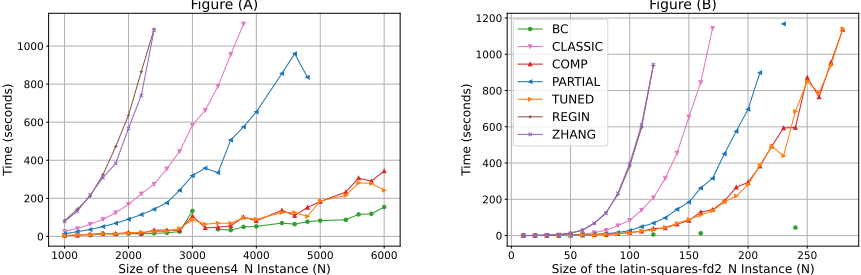
Comparison of the Resolution Time. We compared the resolution times of N-Queens and Latin-Squares, as we can solve most instances within our size range. Figure 5 reports the time in seconds to find the first solution. For each algorithm, a dot represents a solution found. Both problems show that COMP and TUNED are faster than CLASSIC and PARTIAL, up to 14 times faster. This indicates that iterating over unvisited vertices in Bi-BFS and Bi-DFS is in practice much more efficient than iterating over successors, i.e. domains. On N-Queens, BC is 1.65 times faster than TUNED on average, but does not solve queens4 1200 nor queens4 3200. Although the gap is larger on LatinSquares instances solved by BC, the latter hits the time limit on most sizes. This leads us to ask whether our bimodal approach allows GAC to offer a better trade-off than BC.

2 https://github.com/SulianLBC/BimodalAllDiff-IJCAI-2025

3 queens4 model from https://www.hakank.org/minizinc and latin-squares-fd2, langford and golomb models from https://github.com/MiniZinc/minizinc-benchmarks

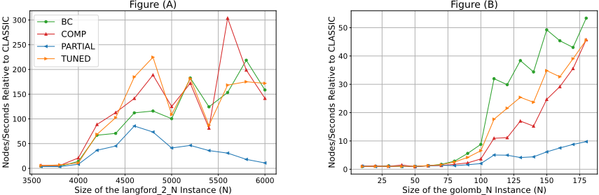
Comparison of the Nodes per Second. To investigate this question, we conduct further experiments on the Langford and Golomb-Ruler problems. All algorithms hit the time limit so we measure branch nodes per second, as in [Tardivo et al., 2023]. In Figure 6, we report the speedup in nodes per second compared to CLASSIC. We choose CLASSIC as the reference algorithm because it has the same implementation as PARTIAL, COMP and TUNED, and it implements R´egin's algorithm while outperforming REGIN and ZHANG. The latter algorithms are not represented because they are slower than the reference algorithm CLASSIC.

To begin with, we observe that COMP and TUNED are comparable to BC in terms of execution time per node on Golomb-Ruler, BC only being about 23% faster on average than TUNED. TUNED is even faster than BC per node on 9 of Langford's 13 instances. This confirms the efficiency of the bimodal approach in the filtering procedure.

Furthermore, the speedup on Golomb-Ruler of COMP and TUNED compared to CLASSIC increases with the size of the instances. The same can be said for Langford, although the curves are less clear. Note that the slope of the PARTIAL curve is explained by its tendency to match CLASSIC's choices in f as size increases, due to Langford's structural properties, leading to a speedup decrease towards 1.

Finally, COMP and TUNED accelerate significantly over CLASSIC, leading to ratios of hundreds on Langford; up to 304 for COMP on langford 2 5600 and 225 for TUNED on langford 2 4800. Also, we observed during the experiments that TUNED was a few dozen times faster per node than CLASSIC on the largest instances of N-Queens; up to 63 times faster on queens4 6000. This is much higher than the 8-fold speedup achieved by GPU optimisations in [Tardivo et al., 2023] on the same range of instances for N-Queens and Langford.

5.2 Empirical Study of Stability

To check stability, we considered instances from MiniZinc Challenge. 4 We selected all models containing at least one ALLDIFFERENT constraint, leading to a total of 242 instances. These instances contain several constraints alongside the ALLDIFFERENT ones, and the latter are not very large. Thus, they are not ideal for studying the asymptotic behaviour of filtering algorithms. So the aim is simply to ensure that our approach does not degenerate compared to the other filtering algorithms.

4 https://github.com/MiniZinc/mzn-challenge, years 2015-2024

We compared BC, ZHANG - the fastest built-in GAC algorithm in Choco-solver, CLASSIC - our implementation of R´egin's algorithm, which served as the reference algorithm in Sect. 5.1, and TUNED - our best performing algorithm on average. We set a 20 minutes (1200 seconds) time limit for the experiments. Among the 242 instances, 72 were solved by at least one algorithmwithin the time limit.

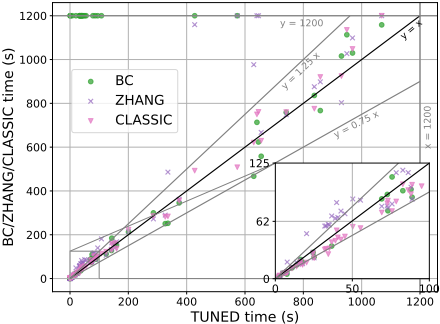
In Figure 7, we compare the resolution times of BC, ZHANG and CLASSIC with TUNED on these 72 instances. A point is represented for each instance and for each algorithm among BC, ZHANG and CLASSIC. The x value is the resolution time of TUNED and the y value is the resolution time of the corresponding algorithm. A point belongs to the x = 1200 vertical line whenever TUNED timed out, while the corresponding algorithm did not. Inversely, a point belongs to the y = 1200 horizontal line whenever the corresponding algorithm timed out, while TUNED did not.

A first comment is that no instances timed out for TUNED but not for any other algorithm. So, we can observe that TUNED did not degenerate on this set of instances. Furthermore, 212 out of the 216 points are above the y = 0.75x line, and no algorithm were more than twice as fast as TUNED on any solved instance. This means that when the considered algorithms were faster than TUNED, they were not by much.

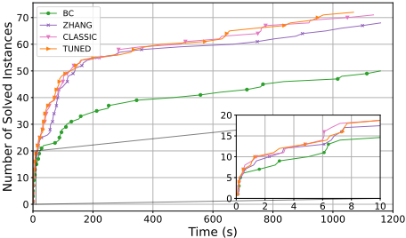
In Figure 8, we show the cumulative number of solved instances by the four algorithms over time. We observe that TUNED solved the most instances (72), CLASSIC solved the second most instances (71) and BC solved the less instances (50). Also, TUNED and CLASSIC seem to dominate the other two, while BC appears to perform less well because of its inability to solve certain easy instances.

5.3 Review of the Experiments

Our experiments show that the bimodal approach, particularly when paired with the TUNED or COMP strategies, significantly improves performance when maintaining GAC for ALLDIFFERENT. More specifically, it outperforms conventional GAC algorithms on problems with large ALLDIFFERENT constraints, and the speedup increases with constraint size. It even resulted in higher ratios than a GPUoptimised approach made for problems with large constraints. Also, the bimodal approach with the TUNED strategy remains competitive on instances with ALLDIFFERENT constraints of bounded size and mixed with numerous other constraints. Finally, the filtering speed of our GAC algorithms is, on most instances, comparable to that of a BC filtering algorithm.

6 Conclusion

The asymptotic analysis of our bimodal approach reveals the potential of our proposal to enhance existing graph algorithms, starting with BFS and DFS. The experimental framework that we propose provides validation of this theoretical result, indicating that the complexity/filtering trade-off of the GAC algorithm is at least equivalent to that of the BC algorithm in terms of efficiency. For this reason, we believe that GAC could now be chosen over BC to filter ALLDIFFERENT

as a default behaviour in CP solvers. To confirm this, further investigation on various problems and instance sizes would be interesting.

Furthermore, our bimodal approach is configurable and opens the way to fine-tuning, as we did with TUNED, to fit better in any CP solver. Also, it can be enhanced with other classical domain operations, such as exploiting knowledge of domain variables' bounds.

Our key contribution lies in Bi-DFS, a faster depth-first search algorithm for CP. Bi-DFS may also be used to improve other constraints, including those based on variablevalue graphs or similar graphs, like CIRCUIT or SAME. We could also use the bimodal approach outside CP when graph representations efficiently implement the iteration and check operations.

Finally, the reason why our graph traversal algorithms BiBFS and Bi-DFS perform so well when iterating over unvisited vertices is because they do not always reach their worst-case time complexities stated in Theorems 1 and 2. In most cases, they are close to their best-case time complexities: Ω(d+ BFS(v)) and Ω(d+ DFS(v)), respectively, for a vertex v when f(v) = FALSE. Theoretically, it would be interesting to identify graph classes where the best-case scenario is always met, or to refine the worst-case complexities with other graph parameters.

Acknowledgments

This publication has emanated from research conducted with the financial support of the Futur & Ruptures program co-granted by IMT, Institut Carnot TSN, Institut Carnot M.I.N.E.S. and Fondation Mines-T´el´ecom.