
Efficient and Rigorous Model-Agnostic Explanations
Proceedings of the Thirty-Fourth International Joint Conference on Artificial Intelligence. Main Track. Pages 2637-2646.
https://doi.org/10.24963/ijcai.2025/294
Keywords
- Constraint Satisfaction and Optimization: CSO: Constraint learning and acquisition
- Constraint Satisfaction and Optimization: CSO: Satisfiabilty
- AI Ethics, Trust, Fairness: ETF: Explainability and interpretability
- Constraint Satisfaction and Optimization: CSO: Constraint programming
Abstract
Explainable artificial intelligence (XAI) is at the core of trustworthy AI. The best-known methods of XAI are sub-symbolic. Unfortunately, these methods do not give guarantees of rigor. Logic-based XAI addresses the lack of rigor of sub-symbolic methods, but in turn it exhibits some drawbacks. These include scalability, explanation size, but also the need to access the details of the machine learning model. Furthermore, access to the details of an ML model may reveal sensitive information. This
paper builds on recent work on symbolic model-agnostic XAI, which is based on explaining samples of behavior of a blackbox ML model, and proposes efficient algorithms for the computation of explanations. The experiments confirm the scalability of the novel algorithms.
- [Amgoud et al., 2023] Leila Amgoud, Philippe Muller, and Henri Trenquier. Leveraging argumentation for generating robust sample-based explanations. In IJCAI, pages 3104- 3111, 2023. IJCAI
- [Amgoud et al., 2024] Leila Amgoud, Martin C. Cooper, and Salim Debbaoui. Axiomatic characterisations of sample-based explainers. In ECAI, pages 770-777, 2024.
- [Audemard et al., 2022] Gilles Audemard, Steve Bellart, Louenas Bounia, Frédéric Koriche, Jean-Marie Lagniez, and Pierre Marquis. On the explanatory power of boolean decision trees. Data Knowl. Eng., 142:102088, 2022.
- [Bach et al., 2015] Sebastian Bach, Alexander Binder, Grégoire Montavon, Frederick Klauschen, Klaus-Robert Müller, and Wojciech Samek. On pixel-wise explanations for non-linear classifier decisions by layer-wise relevance propagation. PloS one, 10(7):e0130140, 2015.
- [Bassan and Katz, 2023] Shahaf Bassan and Guy Katz. To- wards formal XAI: formally approximate minimal expla- nations of neural networks. In TACAS, pages 187-207, 2023.
- [Bendík and Cerná, 2020] Jaroslav Bendík and Ivana Cerná. MUST: minimal unsatisfiable subsets enumeration tool. In TACAS, pages 135-152, 2020.
- [Chikalov et al., 2013] Igor Chikalov, Vadim V. Lozin, Irina Lozina, Mikhail Moshkov, Hung Son Nguyen, Andrzej Skowron, and Beata Zielosko. Three Approaches to Data Analysis -Test Theory, Rough Sets and Logical Analysis of Data, volume 41 of Intelligent Systems Reference Library. Springer, 2013.
- [Cooper and Amgoud, 2023] Martin C. Cooper and Leila Amgoud. Abductive explanations of classifiers under con- straints: Complexity and properties. In ECAI, pages 469- 476, 2023.
- [Cooper and Marques-Silva, 2023] Martin C. Cooper and Joao Marques-Silva. Tractability of explaining classifier decisions. Artif. Intell., 316:103841, 2023.
- [Crama et al., 1988] Yves Crama, Peter L Hammer, and Toshihide Ibaraki. Cause-effect relationships and partially defined boolean functions. Annals of Operations Research, 16:299-325, 1988.
- [Darwiche, 2023] Adnan Darwiche. Logic for explainable AI. In LICS, pages 1-11, 2023.
- [Eiter and Gottlob, 1995] Thomas Eiter and Georg Gottlob. Identifying the minimal transversals of a hypergraph and related problems. SIAM J. Comput., 24(6):1278-1304, 1995.
- [Eiter et al., 2003] Thomas Eiter, Georg Gottlob, and Kazuhisa Makino. New results on monotone dualization and generating hypergraph transversals. SIAM J. Comput., 32(2):514-537, 2003.
- [Eiter et al., 2008] Thomas Eiter, Kazuhisa Makino, and Georg Gottlob. Computational aspects of monotone dualization: A brief survey. Discret. Appl. Math., 156(11):2035-2049, 2008.
- [Fredman and Khachiyan, 1996] Michael L. Fredman and Leonid Khachiyan. On the complexity of dualization of monotone disjunctive normal forms. J. Algorithms, 21(3):618-628, 1996.
- [Gainer-Dewar and Vera-Licona, 2017] Andrew Gainer- Dewar and Paola Vera-Licona. The minimal hitting set generation problem: Algorithms and computation. SIAM J. Discret. Math., 31(1):63-100, 2017.
- [Gorji and Rubin, 2022] Niku Gorji and Sasha Rubin. Suf- ficient reasons for classifier decisions in the presence of domain constraints. In AAAI, pages 5660-5667, 2022.
- [Ignatiev et al., 2019a] Alexey Ignatiev, Nina Narodytska, and Joao Marques-Silva. Abduction-based explanations for machine learning models. In AAAI, pages 1511-1519, 2019.
- [Ignatiev et al., 2019b] Alexey Ignatiev, Nina Narodytska, and Joao Marques-Silva. On validating, repairing and re- fining heuristic ML explanations. CoRR, abs/1907.02509, 2019.
- [Ignatiev, 2020] Alexey Ignatiev. Towards trustable explain- able AI. In IJCAI, pages 5154-5158, 2020. IJCAI
- [Izza and Marques-Silva, 2021] Yacine Izza and João Marques-Silva. On explaining random forests with SAT. In Zhi-Hua Zhou, editor, IJCAI, pages 2584-2591, 2021. IJCAI
- [Izza et al., 2020] Yacine Izza, Alexey Ignatiev, and Joao Marques-Silva. On explaining decision trees. CoRR, abs/2010.11034, 2020.
- [Izza et al., 2022] Yacine Izza, Alexey Ignatiev, and João Marques-Silva. On tackling explanation redundancy in de- cision trees. J. Artif. Intell. Res., 75:261-321, 2022.
- [Karp, 1972] Richard M. Karp. Reducibility among com- binatorial problems. In Raymond E. Miller, James W. Thatcher, and Jean D. Bohlinger, editors, Complexity of Computer Computations, pages 85-103. Springer, 1972.
- [Kavvadias and Stavropoulos, 2005] Dimitris J. Kavvadias and Elias C. Stavropoulos. An efficient algorithm for the transversal hypergraph generation. J. Graph Algorithms Appl., 9(2):239-264, 2005.
- [Koriche et al., 2024] Frédéric Koriche, Jean-Marie Lagniez, Stefan Mengel, and Chi Tran. Learning model agnostic explanations via constraint programming. In ECML, pages 437-453, 2024.
- [Kumar et al., 2020] I.
- Elizabeth Kumar, Suresh Venkata- subramanian, Carlos Scheidegger, and Sorelle A. Friedler. Problems with Shapley-value-based explanations as fea- ture importance measures. In ICML, pages 5491-5500, 2020.
- [Lazo-Cortés et al., 2001] Manuel Lazo-Cortés, José Ruiz- Shulcloper, and Eduardo Alba-Cabrera. An overview of the evolution of the concept of testor. Pattern Recognit., 34(4):753-762, 2001.
- [Lazo-Cortés et al., 2015] Manuel Sabino Lazo-Cortés, José Francisco Martínez Trinidad, Jesús Ariel Carrasco-Ochoa, and Guillermo Sánchez-Díaz. On the relation between rough set reducts and typical testors. Inf. Sci., 294:152- 163, 2015.
- [Liffiton and Malik, 2013] Mark H. Liffiton and Ammar Ma- lik. Enumerating infeasibility: Finding multiple MUSes quickly. In CPAIOR, pages 160-175, 2013.
- [Liffiton and Sakallah, 2008] Mark H. Liffiton and Karem A. Sakallah. Algorithms for computing minimal unsatisfi- able subsets of constraints. J. Autom. Reason., 40(1):1-33, 2008.
- [Lundberg and Lee, 2017] Scott M. Lundberg and Su-In Lee. A unified approach to interpreting model predictions. In NeurIPS, pages 4765-4774, 2017.
- [Malfa et al., 2021] Emanuele La Malfa, Rhiannon Michel- more, Agnieszka M. Zbrzezny, Nicola Paoletti, and Marta Kwiatkowska. On guaranteed optimal robust explanations for NLP models. In IJCAI, pages 2658-2665, 2021. IJCAI
- [Marques-Silva and Huang, 2024] Joao Marques-Silva and Xuanxiang Huang. Explainability is Not a game. Com- mun. ACM, 67(7):66-75, 2024.
- [Marques-Silva and Ignatiev, 2022] Joao Marques-Silva and Alexey Ignatiev. Delivering trustworthy AI through formal XAI. In AAAI, pages 12342-12350, 2022.
- [Marques-Silva, 2022] Joao Marques-Silva. Logic-based ex- plainability in machine learning. In Reasoning Web, pages 24-104, 2022.
- [Pawlak, 1982] Zdzislaw Pawlak. Rough sets. Int. J. Parallel Program., 11(5):341-356, 1982.
- [Ribeiro et al., 2016] Marco Túlio Ribeiro, Sameer Singh, and Carlos Guestrin. "why should I trust you?": Explain- ing the predictions of any classifier. In KDD, pages 1135- 1144, 2016.
- [Ribeiro et al., 2018] Marco Túlio Ribeiro, Sameer Singh, and Carlos Guestrin. Anchors: High-precision model- agnostic explanations. In AAAI, pages 1527-1535, 2018.
- [Rudin and Shaposhnik, 2019] Cynthia Rudin and Yaron Shaposhnik. Globally-consistent rule-based summary- explanations for machine learning models: Application to credit-risk evaluation. SSRN, (3395422), 2019.
- [Rudin and Shaposhnik, 2023] Cynthia Rudin and Yaron Shaposhnik. Globally-consistent rule-based summary- explanations for machine learning models: Application to credit-risk evaluation. J. Mach. Learn. Res., 24:16:1- 16:44, 2023.
- [Serban et al., 2021] Alexandru Constantin Serban, Erik Poll, and Joost Visser. Adversarial examples on object recognition: A comprehensive survey. ACM Comput. Surv., 53(3):66:1-66:38, 2021.
- [Shih et al., 2018] Andy Shih, Arthur Choi, and Adnan Dar- wiche. A symbolic approach to explaining bayesian net- work classifiers. In IJCAI, pages 5103-5111, 2018. IJCAI
- [Wäldchen et al., 2021] Stephan Wäldchen, Jan MacDonald, Sascha Hauch, and Gitta Kutyniok. The computational complexity of understanding binary classifier decisions. J. Artif. Intell. Res., 70:351-387, 2021.
- [Zhang et al., 2024] Hanwei Zhang, Felipe Torres Figueroa, and Holger Hermanns. Saliency maps give a false sense of explanability to image classifiers: An empirical evaluation across methods and metrics. In ACML, 2024.
References were extracted automatically from the PDF and may contain errors.
Full text extracted automatically from the PDF; figures, tables and equations may differ. The PDF is the version of record.
1 Introduction
Explainable artificial intelligence (XAI) seeks to provide human decision-makers with justifications for the predictions made by machine learning (ML) models. As underscored by recent efforts to regulate the deployment of AI models, XAI represents a cornerstone of trustworthy AI. Most efforts on XAI can be characterized as non-symbolic [Bach et al., 2015; Ribeiro et al., 2016; Ribeiro et al., 2018; Lundberg and Lee, 2017]. However, several key limitations of most non-symbolic methods of XAI has been identified in recent years [Ignatiev et al., 2019b; Izza et al., 2020; Kumar et al., 2020; Ignatiev, 2020; Izza et al., 2022; Marques-Silva and Huang, 2024; Zhang et al., 2024]. To address such limitations, logic-based XAI [Shih et al., 2018; Ignatiev et al., 2019a; Izza and Marques-Silva, 2021; W¨aldchen et al., 2021; Malfa et al., 2021; Marques-Silva and Ignatiev, 2022; Audemard et al., 2022; Gorji and Rubin, 2022; Marques-Silva, 2022; Cooper and Marques-Silva, 2023; Darwiche, 2023; Bassan and Katz, 2023] represents a rigorous, model-based, approach to XAI. Although logic-based XAI overcomes the limitations of non-symbolic XAI, it also exhibits some drawbacks. Of these, the most significant are scalability and explanation size. In addition, logic-based XAI is based on the availability of logic encodings of theMLmodel to explain. In some cases this can be challenging, e.g. in the case of support kernel-based support vector machines. Furthermore, logic encodings require access to the full details of ML models. This can represent a major hurdle for logic-based explainability, namely when ML models encode sensitive data.
One key advantage of the best known non-symbolic XAI methods [Ribeiro et al., 2016; Ribeiro et al., 2018; Lundberg and Lee, 2017] is that they are model-agnostic, i.e. these models query the ML model, but the internal details of the model need not be known. Recent work studied logic-based explanations in a model-agnostic setting [Cooper and Amgoud, 2023]. Concretely, the ML model is sampled with the purpose of creating a dataset (i.e. a sample). Alternatively, a dataset could be obtained from training data, or from mixing training data with some sampling of the ML model. In this setting, one important result [Cooper and Amgoud, 2023] is that explanations for why questions (i.e. abductive explanations) can be computed in polynomial time on the size of the dataset. Interest in rigorous sample-based explanations is further illustrated by more recent works [Amgoud et al., 2024; Koriche et al., 2024].
This paper extends the results from [Cooper and Amgoud, 2023] in several ways. First, the paper defines contrastive explanations (i.e. answers to a why not? question) and proves that computing the set of all contrastive explanations is in polynomial time. Second, the paper proposes a novel polynomial-time algorithm for computing one abductive explanation, that improves asymptotically the algorithm outlined in earlier work [Cooper and Amgoud, 2023]. Furthermore, this paper proves several additional results, including the complexity of computing a smallest (i.e. cardinalityminimal) abductive explanation and the complexity of enumerating abductive explanations. In addition, the paper outlines practically efficient algorithms for the enumeration of abductive explanations, and for deciding feature relevancy and necessity. The experimental results confirm the efficiency of the algorithms proposed in the paper, enabling the computation of explanations for fairly large datasets.
The paper is organized as follows. Section 2 introduces the notation and definitions used throughout the paper. Section 3 formalizes sample-based explanations, that represents the model-agnostic approach studied in this paper. Section 4 details novel algorithms for computing sample-based explanations, but also proves complexity results about some of the computational problems related with sample-based explainability. Section 5 analyzes preliminary experimental results, that validate the paper's main claims. Section 6 briefly comments on related work. Finally, Section 7 concludes the paper.
2 Preliminaries
Classification problems. A classification problem is defined on a set of features F = {1, . . . ,m}. Each feature i ∈ F takes values from a domain Di. Features can be categorical or ordinal, and ordinal features can be discrete or realvalued. 1 Feature space F is defined as the cartesian product of the domains of the features, F = D1 × · · · ×Dm. In addition, a classification problem maps feature space into a set of classes K = {c1, . . . , cK}. As a result, a classifier implements a (non-constant) classification function κ : F → K. A classifier is described by the tuple M = (F, F, κ,K). We can refer to the elements of each tuple. For example, the set of features will be denoted by M.F for some M. (When clear from context, then we will just use F). In logic-based XAI, the goal is to explain an instance, given by a point in feature space, v ∈ F and its prediction given κ, c = κ(v).
Finally, the simple model proposed in this section captures some of the best-known and most widely used ML models. Concrete examples, include decision trees, lists and sets, tree ensembles, and (deep) neural networks, among many others.
Logic-based explanations. We adopt the definitions of logic-based explanations used in recent work [Marques-Silva, 2022]. A set of features X ⊆ F is a weak abductive explanation (WAXp) if,
We associate a predicate WAXp with (1), that maps subsets of F to {0, 1}. An abductive explanation (AXp) is a subsetminimal WAXp. Thus, an AXp X is a subset-minimal set of features which suffice to keep the prediction unchanged if their value is unchanged. Similarly, a set of features Y ⊆ F is a weak contrastive explanation (WCXp) if,
We associate a predicate WCXp with (2), that maps subsets of F to {0, 1}. A contrastive explanation (CXp) is a subsetminimal WCXp. Thus, a CXp Y is a subset-minimal set of features that suffice to change the prediction if their value is changed. Hence, a CXp corresponds to an adversarial example [Serban et al., 2021]. The set of all AXps is denoted by A, and the set of all CXps is denoted by C. (The definitions of AXps and CXps are parameterized on the given ML model, and target instance. Since we consider a single ML model and instance, we leave this additional information implicit.)
A feature i ∈ F is relevant if it is included in at least one AXp. A feature is AXp-necessary if it is included in the intersection of all AXps. A feature is CXp-necessary if it is included in the intersection of all CXps.
1 Throughout the paper, and for simplicity, we will assume that features are categorical. However, the extension to non-categorical features is simple, e.g. by using discretization.
| Dec | x1 | x2 | x3 | x4 | κ(·) | ||||||
|---|---|---|---|---|---|---|---|---|---|---|---|
| Dec | x1 | x2 | x3 | x4 | κ(·) | 01 | 0 | 0 | 0 | 1 | 0 |
| 00 | 0 | 0 | 0 | 0 | 0 | 04 | 0 | 1 | 0 | 0 | 0 |
| 02 | 0 | 0 | 1 | 0 | 0 | 05 | 0 | 1 | 0 | 1 | 1 |
| 03 | 0 | 0 | 1 | 1 | 0 | 07 | 0 | 1 | 1 | 1 | 1 |
| 06 | 0 | 1 | 1 | 0 | 0 | 09 | 1 | 0 | 0 | 1 | 0 |
| 08 | 0 | 0 | 1 | 10 | 1 | 0 | 1 | 0 | 0 | ||
| 1 | 0 | 11 | 1 | 0 | 1 | 1 | 0 | ||||
| 12 | 1 | 1 | 0 | 0 | 1 | 13 | 1 | 1 | 0 | 1 | 1 |
| 15 | 1 | 1 | 1 | 1 | 1 | 14 | 1 | 1 | 1 | 0 | 1 |
| (a) Dataset Da ≡ Db1 | (c) Dataset Db2 | ||||||||||
| x1 | 0 | 0 | 0 | 0 | |||||||
| ∈ | {0} 1 | ∈ {1} | 0 | 0 | 1 | 0 | |||||
| 0 | 0 | 1 | 1 | ||||||||
| (b) | 0 2 | Decision | tree | 1 for | Da | (d) | 0 | 1 Reduced | 1 | 0 matrix | Ta |
| 3 | |||||||||||
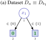
Running example(s). Throughout the paper, we will consider the datasets shown in Fig. 1. From the datasets, we have F = {1, 2, 3, 4}, Di = {0, 1}, with i = 1, 2, 3, 4, K = {0, 1}. Thus, F = {0, 1}4 . Regarding the datasets shown in Fig. 1, the first dataset is Da, as shown. However, the second dataset is composed of Db1 (which matches Da) and Db2 , being denoted by Db. Moreover, the instance considered is: (v, c) = ((1, 1, 1, 1), 1). A decision tree induced fromDa is shown in Fig. 1b. 2
Example 1. Given the DT induced from the dataset Da and the target instance, it is plain that we get A = C = {{1}}, i.e. feature 1 suffices for fixing and changing the prediction.
Samples. Given a classifier defined on some feature space F, a sample S is a subset of F. It is assumed that for each x ∈ S, the prediction can either be computed using the classifier, κ(x), or can be ascribed to x. Throughout, it is assumed that S is finite, with n = |S| the number of points in S. The term dataset denotes a sample such that a prediction is associated with each point in the sample. We will manipulate each sample as a matrix, consisting of m columns, i.e. the features, and n rows, each representing one of the points of the sample. For computing explanations, we will consider the given instance, and the points of the sample with predictions other than the one of the instance. This will be referred to as the reduced matrix. For dataset Da and instance ((1, 1, 1, 1), 1), the resulting reduced matrix is shown in Fig. 1d.
Given an ML model M = (F, F, κ, K), an instance (v, c), and a sample S ⊆ F, an sample-based explanation problem is described by the tuple E = (M, (v, c), S). As before, to refer to the classifier associated with explanation problem E, we will use the notation E.M.κ. (Moreover, and when clear from context, we will just use κ.)
2 Obtained with Orange 3.38.0, https://orangedatamining.com/.
3 Sample-Based Explanations
In this section, we start by revisiting the definition of sample-based (abductive) explanation proposed in recent work [Cooper and Amgoud, 2023; Amgoud et al., 2024]. Afterwards, we introduce additional definitions, and prove some properties of sample-based explanations.
Definitions. Given a sample (or a dataset) S ⊆ F, a samplebased weak abductive explanation (sbWAXp) is a subset of the features X ⊆ F such that,
The predicate sbWAXp : 2F → {0, 1} holds true for the subsets of F for which (3) is true. A subset-minimal sbWAXp is a sample-based AXp (sbAXp). Finally, it is plain that, when S = F, then sbAXps match AXps.
Although not investigated in [Cooper and Amgoud, 2023; Amgoud et al., 2023; Amgoud et al., 2024], sample-based contrastive explanations can also be defined. As a result, given a sample S ⊆ F, a sample-based weak contrastive explanation (sbWCXp) is a subset of features X ⊆ F such that,
The predicate sbWCXp : 2S → {0, 1} holds true for the subsets of F for which (4) is true. A subset-minimal sbWCXp is a sample-based CXp (sbCXp). Clearly, when S = F, then sbCXps match CXps. Moreover, as can be readily concluded, the change in definitions consists of restricting feature space F to the given sample S. Throughout the remainder of the paper, we will use the acronym sbXps to refer to either sbAXps, sbCXps or both.
Regarding the computation of one sbAXp, [Cooper and Amgoud, 2023] outlines a O(m2n) algorithm, where m is the number of features and n is the number of points in S.
Duality of explanations. Several duality results have been proved in logic-based explainability [Marques-Silva, 2022]. In general, each abductive explanation is a minimal hitting set of the set of contrastive explanations, and vice-versa. Similarly, in the case of sbXps, we can prove the following: 3
Proposition 1. (Minimal hitting set duality) Each sbAXp is a minimal hitting set (MHS) of the set of sbCXps, and each sbCXp is a minimal hitting set of the set of sbAXps.
Proof. Each claim is proved separately.
Let X be an sbAXp. Thus, by definition of sbAXp, if the features in X are fixed, then the prediction must be c. Suppose there exists an sbCXp Y such that Y is not hit by X , i.e. X ∩ Y = ∅. Then, by definition of sbCXp, by changing the values of the features in Y, the prediction changes to a value other than c; a contradiction. Thus, each sbAXp X ∈ A must hit each of the sbCXps in C.
3 Observe that, by claiming that an sbAXp X hits some sbCXp Y, it signifies that some feature i ∈ Y is fixed because of X , thereby not allowing Y to be responsible for a change in prediction. Similarly, by claiming that an sbCXp Y hits some sbAXp X, it signifies that some feature i ∈ X is made free due to Y, thereby not allowing X to be responsible for fixing the prediction.
Let Y be an sbCXp. Thus, by definition of sbCXp, if the features in Y are allowed to change their value to some other suitable value, then the prediction changes to a value other than c. Suppose there exists an sbAXp X that is not hit by Y, i.e. Y ∩ X = ∅. Then, by definition of sbAXp, by fixing the values of the features in X , the prediction will remain unchanged; a contradiction. Thus, each sbCXp Y ∈ C must hit each of the sbAXps in A.
An immediate corollary is that each sbAXp must hit each of the sbWCXps, and each sbCXp must hit each of the sbWAXps. Moreover, several of the algorithms described in this paper exploit Proposition 1. These algorithms include the computation of one sbAXp, one smallest sbAXp, the enumeration of sbAXps, but also deciding feature necessity and relevancy [Marques-Silva, 2022].
Sample-based vs. model-based explanations. Let us illustrate the definitions of sample-based explanations.
Example 2. For the dataset Da (see Fig. 1a), it is plain that one sbAXp is {1}. However, given the definition Eq. (3), {2, 4} is also an sbAXp. Thus A = {{1}, {2, 4}}. As a result, by duality, the sbCXps become C = {{1, 2}, {1, 4}}.
Example 3. For the dataset Db (see Figs. 1a and 1c), it is plain that the sbAXps are A = {{1, 2}, {2, 4}}. As a result, by duality, the sbCXps become C = {{2}, {1, 4}}.
As illustrated by Example 1 and Examples 2 and 3, there can exist important differences between model-based explanations and sample-based explanations. A standard algorithm for inducing a decision tree (e.g. CART) must necessarily make assumptions about the points of F not included in S. As can be observed from the induced DT in Fig. 1b, the prediction will be 1 if x1 = 1, and it will be 0 if x1 = 0. However, this may or may not be the case, depending on F \ S. If we consider the complete dataset Db (obtained from joining Db1 = Da and Db2 ), the model-based CXps may be invalid when checked against the complete dataset, since the ML model makes assumptions that may also be invalid, e.g. for the full dataset Db, x1 = 1 does not imply prediction 1.
In contrast, sample-based explanations can offer a more fine-grained characterization. First, sample-based CXps should be viewed as pessimistic, in that no assumptions are made about F\S. Thus, for a sample Sν that includes the starting sample S, S ⊊ Sν , additional features cannot be added to an existing sbCXp. In contrast, features can be removed from an sbCXp. As a result, an sbCXp for S may become a sbWCXp for Sν, when S ⊊ Sν. Second, and in contrast with sbCXps, sbAXps should be viewed as optimistic. Thus, for a sample Sν that includes the starting sample S, S ⊊ Sν, additional features cannot be removed from an existing sbAXp. In contrast, features can be added to an sbAXp. As a result, an sbAXp for S may not be an sbWAXp for Sν , when S ⊊ Sν .
Computing sbWCXps. Given a dataset D, and a target instance (v, cv), each pair point-prediction (u, cu) in the dataset, with cu ̸= cv, encodes an sbWCXp. Clearly, starting from v, and changing the features according to the values of the features in u that differ from those in v, the prediction
Figure 2: (a) Sample-based weak CXps, where 1 means a value that must be changed; (b) Sample-based CXps, i.e. C = {{1, 2}, {1, 4}}.
Figure 3: Example sbCXp matrix yielding exponentially many sbAXps
changes from cv to cu. Thus, the set of sbWCXps, denoted by matrix WC, can be computed as follows. Let u correspond to row j in the reduced matrix. Each such row i is compared with the instance to create row j of matrix WC. For a given feature i, if T[j, i] (representing ui) differs from vi, then WC[j, i] = 1; otherwise WC[j, i] = 0. 4 Thus, the set of sbWCXps is computed in O(mn) time. Furthermore, the features in each sbWCXp j correspond to the entries in row j of WC that take a true value.
Example 4. Fig. 2a illustrates the computation of the set of sbWCXps for dataset Da and the target instance. Thus, WC = {{1, 2, 3, 4}, {1, 2, 4}, {1, 2}, {1, 4}}.
Number of sb(W)CXps. Given the proposed construction of sbWCXps, it is plain that their number is polynomial on the size of the sample. Furthermore, given that each sbCXp is a subset-minimal sbWCXp, then it is also the case that the number of sbCXps is polynomial on the size of the sample. (We will briefly discuss a dedicated algorithm for computing the sbCXps in Section 4.) Thus, the following results hold:
Proposition 2. Both the number of sbWCXps and sbCXps are O(n), where n = |S|, i.e. the size of the sample.
Number of sb(W)AXps. Since each sbAXp is also an sbWAXp, then the number of sbWAXps is no smaller than the number of sbAXps; hence, we only study the number of sbAXps.
Proposition 3. For a sample-based explanation problem E = (M, (v, c), S), the number of sbAXps is worst-case exponential on the size of S.
Example 5. Before proving Proposition 3, we consider the sbCXp matrix shown in Fig. 3, and prove that the number of sbAXps is exponential on the number of sbCXps. For each sbCXp, there are two features to pick from, and we must pick exactly one to hit that sbCXp and to get an subset-minimal set. The number of sbCXps is set to m2 . Thus, the number of sbAXps will be 2 m2 .
4 Given the definition of WAXps/WCXps, in (1), (2) and [Cooper and Amgoud, 2023], two values differ if they are not equal. However, other definitions of value difference could be considered.
Proof. We consider a dataset where each sbWCXp i contains exactly two features 2i - 1 and 2i. Clearly, each sbWCXp is not covered by any other sbWCXp, and so it is an sbCXp. Each sbWAXp is a minimal hitting set of the set of sbCXps. For each i, there are exactly two possible ways to hit the sbCXp i. For the total n = m2 sbCXps, there are 2 m2 possible ways; hence, the number of sbAXps is O(2m).
4 Algorithms &Complexity Results
This section describes algorithms for computing: (i) all sbCXps; (ii) one smallest sbCXp; (iii) one sbAXp; (iv) all sbAXps; and (v) deciding feature necessity and relevancy. This section also proves that the problem of computing one smallest sbAXp is NP-hard, and that the worst-case number of sbAXps is exponential on the size of the sample.
4.1 Algorithms
Enumeration of all sbCXps. From the set of sbWCXps, we can compute the sbCXps as follows. We compare each sbWCXp against all others (in terms of the matrix entries that take value true), and keep the ones having no subsets. This algorithm runs in O(mn2 ). Several low level optimizations can be devised, but these do not change the asymptotic complexity. The rest of the paper assumes that the algorithmwill also associate the number of features with each sbCXp; this adds a constant to the run time of computing sbCXps.
Example 6. For the set of sbWCXps in Fig. 2a, we compare each sbWCXp with every other sbWCXp, with the purpose of finding the subset-minimal. These are shown in Fig. 2b. Thus, C = {{1, 2}, {1, 4}}.
Finding one (smallest) sbCXp. After computing the set of sbCXps, finding a smallest sbCXp just requires traversing the set of sbCXps, and picking one of smallest size. We associate the number of true entries with each sbCXp row, i.e. the sbCXp size, and so the running time is O(n). If the sbCXps have not been computed, then the aggregated run time becomes O(mn2 + n) = O(mn2 ). If the goal is to compute one sbCXp, and the matrix of sbCXps has already been computed, then we simply return any sbCXp. If the matrix of sbCXps has not been computed, then we pick the first sbWCXp, say Y, as the candidate sbCXp, and then iteratively compare with all the other sbWCXps. Each time a sbWCXp N is a proper subset of Y, we replace Y with this new candidate N. Clearly, the run time is O(mn).
Finding one sbAXp. For computing one sbAXp, earlier work [Cooper and Amgoud, 2023] proposed a O(m2n) algorithm. Algorithm 1 proposes an asymptotically more efficient solution, that runs in O(mn) time. Since the sbWCXp matrix takes time O(mn) time to build, then we claim that the proposed algorithm is optimal. Although the algorithm assumes an sbWCXp matrix, it will also produce correct results if the matrix of sbCXps is used. The algorithm works as follows. For an sb(W)CXp in row j, the number of true entries is saved in variable TCs[j]. Each counter denotes the
Algorithm 1 Finding one sbAXp
Input: E: Xp problem; WXp: sbWCXps; TCs: Counts Output: AXp X ⊆ F 1: function oneAXp(E, WXp, TCs) 2: LTCs ←TCs ▷ Local copy of row counters 3: X ← E.M.F ▷ X initialized with all features 4: for i ∈ E.M.F do ▷ Invariant: WAXp(X) holds 5: drop ← true 6: for j ∈ {1, . . . ,WXp.nrows} do 7: if WXp[j, i] then 8: LTCs[j] ← LTCs[j] - 1 9: if LTCs[j] == 0 then ▷ Cannot hit row 10: drop ← false 11: break 12: if drop then 13: X ← X \ {i} ▷ AXp will not include i 14: else ▷ Invariant: ¬WAXp(X \ {i}) holds 15: for k ∈ {1, . . . , j} do ▷ Recover counters 16: if WXp[k, i] then 17: LTCs[k] ← LTCs[k] + 1 18: return X ▷ AXp(X ) holdsnumber of features hitting that row. The algorithm iteratively drops features from a reference set X, and decrements the row counters. When the counter for row j reaches 0, then no features hit row j, and so X \ {i} would no longer represent an sbWAXp. In that case, the feature cannot be removed from set X, and the decremented counters need to be recovered. If no decremented counter reaches 0, then feature i is removed from X, since X \ {i} still represents an sbWAXp. Thus, the algorithm's complexity is O(mn). A simple optimization that does not reduce the worst-case run time is to replace the matrix of sbWCXps with the matrix of sbCXps. However, this requires pre-computing the matrix of sbCXps.
Example 7. Table 1 summarizes the computation of one sbAXp for the running example, taking into account the matrix of sbCXps shown in Fig. 2b. Given the picked order of the features, i.e. ⟨1, 2, 3, 4⟩, the computed sbAXp is {2, 4}. Using a different order, a different sbAXp might be obtained. For example, given the order ⟨2, 3, 4, 1⟩, then the computed sbCXp would be {1}. From Proposition 1, we know that each sbAXp is a MHS of the set of sbCXps, and vice-versa.
Finding one smallest sbAXp. As proved in Section 4.2, finding one smallest sbAXp is computationally hard, and unlikely to be solved in polynomial time. Nevertheless, it is simple to devise a logic encoding for computing smallest sbAXps. We encode the problem to propositional maximum satisfiability (MaxSAT). The proposed encoding can start from the matrix of sbWCXps or the matrix of sbCXps; we will refer to the corresponding matrix as MC. We associate a boolean variable pi with each each feature i ∈ F, P = {pi | i ∈ F}. Furthermore, for a (W)CXp represented by row j, let F(j) denote the set of features i such that MC[j, i] is true. Then, for each j, we create the constraint,
i.e., we must pick one of the features so as to hit the sb(W)CXp. The constraints above represent the background knowledge, i.e. the hard constraints that must be consistent. In addition, we encode a preference for not assigning the pi variables to true. Thus, the soft constraints are of the form (¬pi). Clearly, the encoding is polynomial on the size of the sbWCXps/sbCXps matrices.
Example 8. For the set of sbCXps in Fig. 2b, the hard (H) and the soft (S) constraints become,
Let ν : P → {0, 1} denote a valuation of the pi variables. Clearly, the minimum number of falsified soft constraints is 1, by setting ν(p1) = 1, that satisfies all the hard constraints, and allows setting the value of the other variables to 0, i.e. ν(p2) = ν(p3) = ν(p4) = 0.
Enumeration of sbAXps. Given that the set of all sbCXps can be computed in polynomial-time, there is no need for the concurrent enumeration of sbAXps and sbCXps, e.g. using a MARCO-like algorithm [Liffiton and Malik, 2013; Bend´ık and Cern´a, 2020]. As a result, we can either exploit theoretically efficient algorithms [Fredman and Khachiyan, 1996], which provide quasi-polynomial time guarantees on the size of the input and output, use existing algorithms for computing minimal hitting sets [Kavvadias and Stavropoulos, 2005; Liffiton and Sakallah, 2008; Gainer-Dewar and Vera-Licona, 2017], or consider a logic encoding. Given the algorithms described above, a simple solution is to enumerate smallest sbAXps, by increasing size.
Feature necessity & relevancy. Due to minimal hitting set duality, feature relevancy can be decided using the set of sbCXps. Thus, the overall running time will be O(mn2 ). If the set of spCXps is known, then deciding feature relevancy requires traversing one column of the sbCXp matrix, in O(n) time. For finding all the sbCXp-necessary features, it suffices to compute the intersection of all sbCXps. Given that there can exist O(n) and each sbCXp has O(m) features, then sbCXp-necessity can be computed with O(n) intersections, each involving O(m) elements. Hence, the running time is in O(mn), but with time O(mn2 ) for computing the sbCXps. For finding all the sbAXp-necessary features, it would be infeasible to intersect all the sbAXps, since their number is worst-case exponential. However, it is simple to conclude that any feature that occurs in all sbAXps represents an sbCXp of size 1. Hence, spAXp-necessity is decided by computing the sbCXps of size 1. For this, we need to compute all the sbCXps in O(mn2 ) time, and then traverse the sbCXps in O(n) time. Observe that there will be no need to traverse the rows if the number of true entries is associated with each row; hence the run time complexity follows.
Example 9. For the set of sbCXps of Fig. 2b, it is clear that features 1, 2, 4 are relevant, feature 1 is sbCXp-necessary, and that there are no sbAXp-necessary features.
A complete example. Given Db from Figs. 1a and 1c, we compute the reduced matrix, then the sbWCXp matrix WC,b, and finally the sbCXp matrix Cb, that is shown in Fig. 4a. The
| Starting X | Start. [LTCs[1], LTCs[2]] | Feature | Temp. [LTCs[1], LTCs[2]] | Decision | Updated X |
|---|---|---|---|---|---|
| {1, 2, 3, 4} | [2, 2] | 1 | [1, 1] | Drop 1 | {2, 3, 4} |
| {2, 3, 4} | [1, 1] | 2 | [0, 1] | Keep 2 | {2, 3, 4} |
| {2, 3, 4} | [1, 1] | 3 | [1, 1] | Drop 3 | {2, 4} |
| {2, 4} | [1, 1] | 4 | [1, 0] | Keep 4 | {2, 4} |
| Problem | Complexity | |
|---|---|---|
| Total | Given sbCXps | |
| All sbCXps | O(mn2 ) | - |
| One sbCXp | O(mn) | O(1) |
| One (smallest) sbCXp | O(mn2 ) | O(n) |
| One sbAXp | O(mn) | O(mn) |
| Feature relevancy | O(mn2 ) | O(n) |
| sbAXp-necessity | O(mn2 ) | O(mn) |
| sbCXp-necessity | O(mn2 ) | O(n) |
Table 2: Complexity of tractable sbXp problems
algorithms described earlier in this section can then be used for computing the sbCXp matrix shown in Fig. 4a, and also one sbAXp, and enumeration of sbAXps. These are shown in Fig. 4b. Finally, we can conclude the following: (i) features 1, 2 and 4 are relevant, because these features occur in some sbCXp; (ii) feature 3 is irrelevant, because it does not occur in any sbCXp; (iii) there are no sbCXp-necessary features, since the intersection of sbCXps is empty; and (iv) there is one sbAXp-necessary feature, namely 2, because there exists a sbCXp of size 1 composed of feature 2.
Summary. Table 2 summarizes the complexity results discussed in this section for tractable problems related with sample-based explanations. The following section discusses intractability results.
4.2 Complexity Results
Complexity-wise, we consider two problems: (i) enumeration of sbAXps; and (ii) finding one smallest sbAXp.
Enumeration of sbAXps. The problem of enumerating sbAXps maps to several other well-known computational problems, namely monotone dualization [Fredman and Khachiyan, 1996; Eiter et al., 2008] and computing the transversal of an hypergraph [Eiter and Gottlob, 1995; Kavvadias and Stavropoulos, 2005; Liffiton and Sakallah, 2008]. Moreover, the connections between these two problems are well-known [Eiter et al., 2003]. A seminal result is the quasipolynomial algorithm of Fredman and Khachiyan [Fredman and Khachiyan, 1996] on the size of input and output. The following result equates sbAXp enumeration with monotone dualization and computing hypergraph transversals.
Proposition 4. The problem of computing the transversal on an hypergraph reduces to sbAXp enumeration.
Proof. (Sketch) Each hyperedge maps to an sbCXp. The minimal hitting sets of the sbCXps represent the hyperedges of the hypergraph transversal.
Finding one smallest sbAXp. We prove that deciding the existence of a sbAXp with size no larger than k is NPcomplete.
Proposition 5. The problem of deciding the existence of an sbAXp of size no larger than k is NP-complete.
Proof. The decision problem is in NP. By guessing a possible sbAXp with size no larger than k, one can check in polynomial time whether all rows of the sbCXp matrix are hit.
To prove NP-hardness, we reduce a well-known NP-complete decision problem to our target problem. For that, we choose the decision version of the set covering problem, which is well-known to be NP-complete [Karp, 1972]. Given a set U, and a set V = {V1, . . . , VK} of subsets of U, the set-covering decision problem is to decide the existence of at most k sets in V such that their union is U, in which case we say that U has a k-cover given V .
We reduce the set-covering to finding an sbAXp of at most size k as follows, by creating a suitable matrix M. Each row represents one element of U. For element j of U, M[j, i] = 1 if element j is included in Vi. Clearly, the construction of M is in polynomial time. Moreover, it is simple to prove that there exists a k-cover of U if and only if there exists an sbAXp of size no greater than k.
5 Experiments
This section presents results on the algorithms proposed in the paper. We opt to explain existing large-size datasets. However, as argued in Section 1, we could have sampled ML models, or could even mix the two.
Experimental setup. The experiments consider 30 realworld datasets. The number of samples range from 1000 to over one million, whereas the number of features range from 10 to 250. All datasets are concerned with solving supervised classification problems, that include different types of features (boolean, categorical, integer and real values). Also, for each dataset, 10 different instances were randomly selected; in the experiments, the mean values are reported.
In the experiments, we measured the time required to compute: (i) one sbCXp; (ii) all sbCXps; (iii) one sbAXp; (iv) one smallest sbAXp; (v) several sbAXps; and (vi) feature relevancy & necessity (for sbAXps/sbCXps). All experiments were conducted on a computer with an AMD Ryzen™ 7 4800HS and 16 GB of RAM.
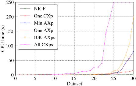
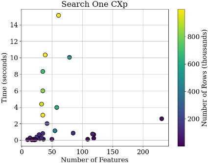
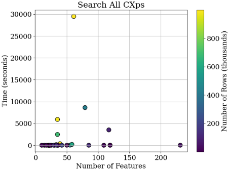
Computing sbCXps. As detailed in Section 3, the computation of the set of sbWCXps is a crucial step for identifying sbCXps. As also noted in Section 3, one must define when values should be deemed equal or not. In this paper, we opted for the equality operator, given the proposed definition of (sb)AXps/(sb)CXps. Once the set of sbWCXps is computed, finding one or all sbCXps can be attained by using the algorithms detailed in Section 4.1. The time required to find one sbCXp was measured starting from the set of sbWCXps and not from the set of sbCXps. Fig. 5 shows the distribution of running times for computing both a single sbCXp (red) and for computing all sbCXps (pink). Motivated by the sizes of the datasets considered, the time taken for computing all sbCXps can be significant, but it exceeds 250s only for seven datasets. The maximum time for finding one sbCXp and all sbCXps was 16.3s and 31176s, respectively. Figure 6 shows in more detail the behavior for the case of computing one sbCXP in Figure 6a and all sbCXps in Figure 6b, respectively. In each plot, each dot represents the result for a single dataset, and the color intensity (shading towards yellow) indicates the number of rows in the tested dataset. This allows us to highlight the impact of the number of rows and columns on the evaluated algorithms. We can notice here, that the algorithm for finding a single sbCXp is more sensitive to the number of rows in the dataset. A similar pattern occurs for the algorithm for finding all sbCXps, but with a more pronounced impact. This is to be expected, as both algorithms require identifying the set of all sbWCXps.
Computing sbAXps. As noted in Section 4.1, we can exploit minimal hitting set duality for computing one sbAXp using the set of sb(W)CXps. In the experiments, a single sbAXp and a smallest sbAXp were computed starting from set of sbCXps. Fig. 5 shows the the time required to find a single sbAXp (brown), a smallest sbAXp (violet), and also ten thousand (10k) sbAXps (yellow).As was mentioned before, the time required to get all sbCXps in order to run the
(a) Find one sbCXp
(b) Find all sbCXps
Figure 6: Finding sbCXps
algorithms is measured separately. Section 4.2 proves that finding one smallest sbAXp is computationally hard, and so it is expected to require more time in practice. The smallest sbAXp trivial cases (columns with only value 1 in the sbCXp set) were removed from the sbCXp set beforehand, as an additional optimization. In the experimentation, the computation of a single sbAXp and a smallest sbAXp have a similar running time. For the selected datasets, the maximum time for computing one (resp. smallest) sbAXp was 71.3s (resp. 66.8s). As noted also in Section 4.2, we adapt the finding of smallest sbAXps in order to enumerate the selected number of sbAXps (this also means that sbAXps are enumerated by increasing size). The maximum enumeration time was 139.2s.
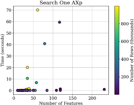
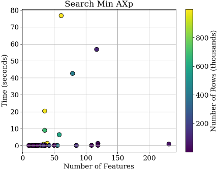
(b) Find a smallest sbAXp
Figure 7: Finding sbAXps
The choice of 10K sbAXps aims solely at illustrating the scalability of the proposed algorithm. Despite the fairly small limit on the number of sbAXps to be enumerated, as proved in Section 3 the worst-case is exponential on the number of features. Figure 7 shows the relationship between running time, number of features and number of rows. Here, we have in Figure 7a for finding one sbAXp and, in Figure 7a, for finding a smallest sbAXp.
Feature relevance, sbAXp and sbCXp necessity. As argued in Section 4.1, deciding feature relevancy and necessity only requires analysis of the set of sbCXps. For simplicity, we opted to aggregate the running times for deciding relevancy and necessity, not including the time for search all sbCXps. As shown in Fig. 5, the running times for finding relevant and necessary features (green) is in general negligible, even for fairly large datasets. The maximum time reported for the tested datasets was 1.12s.
6 RelatedWork
In logic-based XAI, sample-based explanations were introduced in recent work [Cooper and Amgoud, 2023]. Additional recent efforts include [Amgoud et al., 2024; Koriche et al., 2024]. A related line of work focused on smallest explanations [Rudin and Shaposhnik, 2019; Rudin and Shaposhnik, 2023]. Nevertheless, the analysis of tabular data has been studied in different domains, including rough sets (RS) [Pawlak, 1982], logic analysis of data (LAD) [Crama et al., 1988], and testor theory (TT) [Lazo-Cort´es et al., 2001], among others. The connections between these approaches to data analysis have been the subject of past research [Chikalov et al., 2013; Lazo-Cort´es et al., 2015]. Some of the concepts used in RS, LAD and TT mimic those proposed in samplebased in XAI [Cooper and Amgoud, 2023]. For example, the algorithms for computing one or all sbCXps proposed in this paper find equivalent in earlier work on RS, LAD or TT. To the best of our knowledge, the algorithms for finding either one subset-minimal sbAXp or one cardinality-minimal sbAXp are novel, and improve on earlier proposals. The same holds true for the complexity results developed in this paper. As noted above, the work of [Rudin and Shaposhnik, 2019; Rudin and Shaposhnik, 2023] focused on smallest explanations for the given sample. This approach exploits a setcovering formulation, but does not analyze the complexity of the problem; it also overlooks the polynomial-time cases.
7 Conclusions &Research Directions
Logic-based XAI addresses important limitations of subsymbolic XAI, providing explanations that are model-based and so model-accurate. However, logic-based XAI requires logic encodings of ML models, and this raises a few challenges, including scalability, but also the need to access the ML model being explained. In some situations, such ML models are not readily available for analysis. One alternative is sample-based XAI [Cooper and Amgoud, 2023], which builds on the sampled behavior of the ML model for computing rigorous logic-based explanations.
This paper proposes novel algorithms for computing sample-based abductive and contrastive explanations, for the enumeration of explanations, but also for deciding feature necessity and relevancy. The paper also proves complexity results regarding the computation of sample-based explanations. The experimental results confirm the scalability of the algorithms proposed in the paper. A number of research directions can be envisioned. For example, future work will extend the algorithms proposed in this paper to the cases of non-categorical and non-tabular data.
Acknowledgments
This work was supported in part by the Spanish Government under grants PID 2023-152814OB-I00, PCI 2022135010-2, PID 2022-139835NB-C21, PIE 2023-5AT010, HE-101070930, and by ICREA starting funds. The first author (JMS) also acknowledges the extra incentive provided by the ERC in not funding this research.
@inproceedings{ijcai2025p294,
  title     = {Efficient and Rigorous Model-Agnostic Explanations},
  author    = {Marques-Silva, Joao and Lefebre-Lobaina, Jairo A. and Martínez, María Vanina},
  booktitle = {Proceedings of the Thirty-Fourth International Joint Conference on
               Artificial Intelligence, {IJCAI-25}},
  publisher = {International Joint Conferences on Artificial Intelligence Organization},
  editor    = {James Kwok},
  pages     = {2637--2646},
  year      = {2025},
  month     = {8},
  note      = {Main Track},
  doi       = {10.24963/ijcai.2025/294},
  url       = {https://doi.org/10.24963/ijcai.2025/294},
}
TY - CPAPER TI - Efficient and Rigorous Model-Agnostic Explanations AU - Marques-Silva, Joao AU - Lefebre-Lobaina, Jairo A. AU - Martínez, María Vanina T2 - Proceedings of the Thirty-Fourth International Joint Conference on Artificial Intelligence, IJCAI-25 PB - International Joint Conferences on Artificial Intelligence Organization PY - 2025 SP - 2637 EP - 2646 DO - 10.24963/ijcai.2025/294 UR - https://doi.org/10.24963/ijcai.2025/294 ER -Copied
Machine-readable versions of this paper, for tools and AI agents:





