
New Algorithms for #2-SAT and #3-SAT
Proceedings of the Thirty-Fourth International Joint Conference on Artificial Intelligence. Main Track. Pages 2666-2674.
https://doi.org/10.24963/ijcai.2025/297
Keywords
- Constraint Satisfaction and Optimization: CSO: Satisfiabilty
Abstract
The #2-SAT and #3-SAT problems involve counting the number of satisfying assignments (also called models) for instances of 2-SAT and 3-SAT, respectively. In 2010, Zhou et al. (https://doi.org/10.1609/aaai.v24i1.7537) proposed an O*(1.1892^m)-time algorithm for #2-SAT and an efficient approach for #3-SAT, where m denotes the number of clauses. In this paper, we show that the weighted versions of #2-SAT and #3-SAT can be solved in O*(1.1082^m) and O*(1.4423^m) time, respectively. These results directly apply to the unweighted cases and achieve substantial improvements over the previous results. These advancements are enabled by the introduction of novel reduction rules, a refined analysis of branching operations, and the application of path decompositions on the primal and dual graphs of the formula.
- [Bacchus et al., 2003] Fahiem Bacchus, Shannon Dalmao, and Toniann Pitassi. Algorithms and complexity results for #sat and bayesian inference. In 44th Symposium on Foun- dations of Computer Science (FOCS 2003), 11-14 October 2003, Cambridge, MA, USA, Proceedings, pages 340-351. IEEE Computer Society, 2003.
- [Beigel and Eppstein, 2005] Richard Beigel and David Epp- stein. 3-coloring in time o(1.3289 n ). J. Algorithms, 54(2):168-204, 2005.
- [Biere et al., 2021] Armin Biere, Marijn Heule, Hans van Maaren, and Toby Walsh, editors. Handbook of Satisfiabil- ity -Second Edition, volume 336 of Frontiers in Artificial Intelligence and Applications. IOS Press, 2021.
- [Chavira and Darwiche, 2008] Mark Chavira and Adnan Darwiche. On probabilistic inference by weighted model counting. Artif. Intell., 172(6-7):772-799, 2008.
- [Chu et al., 2021] Huairui Chu, Mingyu Xiao, and Zhe Zhang. An improved upper bound for SAT. In Thirty-Fifth AAAI Conference on Artificial Intelligence, AAAI 2021, Thirty-Third Conference on Innovative Applications of Ar- tificial Intelligence, IAAI 2021, The Eleventh Symposium on Educational Advances in Artificial Intelligence, EAAI 2021, Virtual Event, February 2-9, 2021, pages 3707- 3714. AAAI Press, 2021.
- [Cook, 1971] Stephen A. Cook. The complexity of theorem- proving procedures. In Michael A. Harrison, Ranan B. Banerji, and Jeffrey D. Ullman, editors, Proceedings of the 3rd Annual ACM Symposium on Theory of Comput- ing, May 3-5, 1971, Shaker Heights, Ohio, USA, pages 151-158. ACM, 1971.
- [Cygan et al., 2016] Marek Cygan, Holger Dell, Daniel Lokshtanov, Dániel Marx, Jesper Nederlof, Yoshio Okamoto, Ramamohan Paturi, Saket Saurabh, and Mag- nus Wahlström. On problems as hard as CNF-SAT. ACM Trans. Algorithms, 12(3):41:1-41:24, 2016.
- [Dahllöf et al., 2005] Vilhelm Dahllöf, Peter Jonsson, and Magnus Wahlström. Counting models for 2sat and 3sat formulae. Theor. Comput. Sci., 332(1-3):265-291, 2005.
- [Dubois, 1991] Olivier Dubois. Counting the number of so- lutions for instances of satisfiability. Theor. Comput. Sci., 81(1):49-64, 1991.
- [Dudek et al., 2020] Jeffrey M. Dudek, Vu H. N. Phan, and Moshe Y. Vardi. DPMC: weighted model counting by dynamic programming on project-join trees. In Helmut Simonis, editor, Principles and Practice of Constraint Programming -26th International Conference, CP 2020, Louvain-la-Neuve, Belgium, September 7-11, 2020, Pro- ceedings, volume 12333 of Lecture Notes in Computer Sci- ence, pages 211-230. Springer, 2020.
- [Dueñas-Osorio et al., 2017] Leonardo Dueñas-Osorio, Kuldeep S. Meel, Roger Paredes, and Moshe Y. Vardi. Counting-based reliability estimation for power- transmission grids. In Satinder Singh and Shaul Markovitch, editors, Proceedings of the Thirty-First AAAI Conference on Artificial Intelligence, February 4-9, 2017, San Francisco, California, USA, pages 4488-4494. AAAI Press, 2017.
- [Fichte et al., 2019] Johannes Klaus Fichte, Markus Hecher, and Markus Zisser. An improved gpu-based SAT model counter. In Thomas Schiex and Simon de Givry, editors, Principles and Practice of Constraint Programming -25th International Conference, CP 2019, Stamford, CT, USA, September 30 -October 4, 2019, Proceedings, volume 11802 of Lecture Notes in Computer Science, pages 491- 509. Springer, 2019.
- [Fichte et al., 2022] Johannes Klaus Fichte, Markus Hecher, Patrick Thier, and Stefan Woltran. Exploiting database management systems and treewidth for counting. Theory Pract. Log. Program., 22(1):128-157, 2022.
- [Fichte et al., 2023a] Johannes Klaus Fichte, Daniel Le Berre, Markus Hecher, and Stefan Szeider. The silent (r)evolution of SAT. Commun. ACM, 66(6):64-72, 2023.
- [Fichte et al., 2023b] Johannes Klaus Fichte, Markus Hecher, Michael Morak, Patrick Thier, and Stefan Woltran. Solving projected model counting by utilizing treewidth and its limits. Artif. Intell., 314:103810, 2023.
- [Fomin and Kratsch, 2010] Fedor V. Fomin and Dieter Kratsch. Exact Exponential Algorithms. Texts in The- oretical Computer Science. An EATCS Series. Springer, 2010.
- [Fomin et al., 2009] Fedor V. Fomin, Serge Gaspers, Saket Saurabh, and Alexey A. Stepanov. On two techniques of combining branching and treewidth. Algorithmica, 54(2):181-207, 2009.
- [Gaspers and Sorkin, 2009] Serge Gaspers and Gregory B. Sorkin. A universally fastest algorithm for max 2-sat, max 2-csp, and everything in between. In Claire Mathieu, edi- tor, Proceedings of the Twentieth Annual ACM-SIAM Sym- posium on Discrete Algorithms, SODA 2009, New York, NY, USA, January 4-6, 2009, pages 606-615. SIAM, 2009.
- [Gomes et al., 2021] Carla P. Gomes, Ashish Sabharwal, and Bart Selman. Model counting. In Armin Biere, Mar- ijn Heule, Hans van Maaren, and Toby Walsh, editors, Handbook of Satisfiability -Second Edition, volume 336 of Frontiers in Artificial Intelligence and Applications, pages 993-1014. IOS Press, 2021.
- [Hecher et al., 2020] Markus Hecher, Patrick Thier, and Ste- fan Woltran. Taming high treewidth with abstraction, nested dynamic programming, and database technology. In Luca Pulina and Martina Seidl, editors, Theory and Ap- plications of Satisfiability Testing -SAT 2020 -23rd In- ternational Conference, Alghero, Italy, July 3-10, 2020, Proceedings, volume 12178 of Lecture Notes in Computer Science, pages 343-360. Springer, 2020.
- [Impagliazzo and Paturi, 2001] Russell Impagliazzo and Ra- mamohan Paturi. On the complexity of k-SAT. J. Comput. Syst. Sci., 62(2):367-375, 2001.
- [Iwama, 1989] Kazuo Iwama. CNF satisfiability test by counting and polynomial average time. SIAM J. Comput., 18(2):385-391, 1989.
- [Korhonen and Järvisalo, 2021] Tuukka Korhonen and Matti Järvisalo. Integrating tree decompositions into decision heuristics of propositional model counters (short paper).
- In Laurent D. Michel, editor, 27th International Confer- ence on Principles and Practice of Constraint Program- ming, CP 2021, Montpellier, France (Virtual Conference), October 25-29, 2021, volume 210 of LIPIcs, pages 8:1- 8:11. Schloss Dagstuhl -Leibniz-Zentrum für Informatik, 2021.
- [Kutzkov, 2007] Konstantin Kutzkov. New upper bound for the #3-sat problem. Inf. Process. Lett., 105(1):1-5, 2007.
- [Lozinskii, 1992] Eliezer L. Lozinskii. Counting proposi- tional models. Inf. Process. Lett., 41(6):327-332, 1992.
- [Narodytska et al., 2019] Nina Narodytska, Aditya A. Shrotri, Kuldeep S. Meel, Alexey Ignatiev, and João Marques-Silva. Assessing heuristic machine learning explanations with model counting. In Mikolás Janota and Inês Lynce, editors, Theory and Applications of Satisfiability Testing -SAT 2019 -22nd International Conference, SAT 2019, Lisbon, Portugal, July 9-12, 2019, Proceedings, volume 11628 of Lecture Notes in Computer Science, pages 267-278. Springer, 2019.
- [Roth, 1996] Dan Roth. On the hardness of approximate rea- soning. Artif. Intell., 82(1-2):273-302, 1996.
- [Samer and Szeider, 2010] Marko Samer and Stefan Szeider. Algorithms for propositional model counting. J. Discrete Algorithms, 8(1):50-64, 2010.
- [Sang et al., 2005] Tian Sang, Paul Beame, and Henry A. Kautz. Performing bayesian inference by weighted model counting. In Manuela M. Veloso and Subbarao Kambham- pati, editors, Proceedings, The Twentieth National Confer- ence on Artificial Intelligence and the Seventeenth Innova- tive Applications of Artificial Intelligence Conference, July 9-13, 2005, Pittsburgh, Pennsylvania, USA, pages 475- 482. AAAI Press / The MIT Press, 2005.
- [Valiant, 1979] Leslie G. Valiant. The complexity of com- puting the permanent. Theor. Comput. Sci., 8:189-201, 1979.
- [Wahlström, 2008] Magnus Wahlström. A tighter bound for counting max-weight solutions to 2sat instances. In Martin Grohe and Rolf Niedermeier, editors, Parameterized and Exact Computation, Third International Workshop, IW- PEC 2008, Victoria, Canada, May 14-16, 2008. Proceed- ings, volume 5018 of Lecture Notes in Computer Science, pages 202-213. Springer, 2008.
- [Xiao, 2022] Mingyu Xiao. An exact maxsat algorithm: Fur- ther observations and further improvements. In Luc De Raedt, editor, Proceedings of the Thirty-First International Joint Conference on Artificial Intelligence, IJCAI 2022, Vienna, Austria, 23-29 July 2022, pages 1887-1893. ij- cai.org, 2022. IJCAI
- [Zhang, 1996] Wenhui Zhang. Number of models and satisfiability of sets of clauses. Theor. Comput. Sci., 155(1):277-288, 1996.
- [Zhou et al., 2010] Junping Zhou, Minghao Yin, and Chun- guang Zhou. New worst-case upper bound for #2-sat and #3-sat with the number of clauses as the parameter. In Maria Fox and David Poole, editors, Proceedings of the Twenty-Fourth AAAI Conference on Artificial Intelligence, AAAI 2010, Atlanta, Georgia, USA, July 11-15, 2010, pages 217-222. AAAI Press, 2010.
References were extracted automatically from the PDF and may contain errors.
Full text extracted automatically from the PDF; figures, tables and equations may differ. The PDF is the version of record.
1 Introduction
The BOOLEAN SATISFIABILITY problem (SAT), the first problem to be proven NP-complete [Cook, 1971], is a cornerstone of computational complexity theory. Its counting variant, the PROPOSITIONAL MODEL COUNTING problem (#SAT), introduced and shown to be #P-complete by Valiant (1979), holds comparable significance.
Given a CNF formula, SAT seeks to determine whether the formula is satisfiable, while #SAT aims to count the number of satisfying assignments (also known as models). Both SAT and #SAT, along with their variants, are among the most influential problems in computational theory due to their broad applications in computer science, artificial intelligence, and numerous other domains, both theoretical and practical. As such, these problems have garnered substantial attention and have been extensively studied across various fields, including computational complexity and algorithm design. For comprehensive surveys, For comprehensive surveys, we refer to [Biere et al., 2021; Fichte et al., 2023a].
This paper focuses on #SAT and its weighted extension, WEIGHTED MODEL COUNTING (WMC, or weighted #SAT). In WMC, each literal (a variable or its negation) in the formula is assigned a weight. The task is to compute the sum of the weights of all satisfying assignments, where the weight of an assignment is the product of the weights of its literals. Notably, WMC reduces to #SAT when all literals have identical weights. Efficient algorithms for (weighted) #SAT have a profound impact on various application areas [Gomes et al., 2021], such as probabilistic inference [Roth, 1996; Bacchus et al., 2003; Sang et al., 2005; Chavira and Darwiche, 2008], network reliability estimation [Due˜nas-Osorio et al., 2017], and explainable AI [Narodytska et al., 2019]. This significance is highlighted by the annual Model Counting Competition 1 , which bridges theoretical advancements and practical implementations in model counting.
∗Corresponding Author
A fundamental question is: how fast (weighted) #SAT can be solved in the worst case? The na¨ıve algorithm, which enumerates all assignments, runs in O∗ (2n ) time 2 , where n is the number of variables in the formula. Under the Strong Exponential Time Hypothesis (SETH) [Impagliazzo and Paturi, 2001], SAT (and thus #SAT) cannot be solved in O∗ ((2-ϵ)n ) time for any constant ϵ > 0. Another key parameter, the number of clauses m in the formula, has also been extensively studied. It is well-known that #SAT can be solved in O∗ (2m) time using the Inclusion-Exclusion principle [Iwama, 1989; Lozinskii, 1992], which also applies to the weighted variant. However, no algorithm with a runtime of O∗ (cm) for c < 2 was discovered. In fact, Cygan et al. (2016) proved that such an algorithm does not exist unless SETH fails.
The barriers 2n and 2m can be broken for restricted versions of (weighted) #SAT. One notable example is the (weighted) #k-SAT problem, where each clause contains at most k literals. There is a rich history of faster algorithms for #2-SAT and #3-SAT [Dubois, 1991; Zhang, 1996; Dahll¨of et al., 2005; Kutzkov, 2007; Wahlstr¨om, 2008; Zhou et al., 2010]. The current fastest algorithms for weighted #2-SAT and #3-SAT achieve runtimes of O∗ (1.2377n ) [Wahlstr¨om, 2008] and O∗ (1.6423n ) [Kutzkov, 2007], respectively. For the parameter m, Zhou et al. introduced an O∗ (1.1740m)- time algorithm for #2-SAT and suggested a simple approach for #3-SAT. However, the analysis of the #3-SAT algorithm in [Zhou et al., 2010] does not yield a valid runtime bound.
Our Contribution. We propose two novel algorithms, Alg2CNF and Alg3CNF, for weighted #2-SAT and weighted #3-SAT, achieving runtime bounds of O∗ (1.1082m) and O∗ (1.4423m), respectively. The algorithms and complexity bounds directly apply to the unweighted case, significantly improving upon previous results. To this end, we bring new techniques for (weighted) #2-SAT and #3-SAT.
2 The O∗ notation suppresses polynomial factors in the input size.
Our Approach. Most existing algorithms, including ours, are classical branch-and-search algorithms (also called DPLL-style algorithms) that first apply reduction (preprocessing) rules and then recursively solve the problem via branching (e.g., selecting a variable and assigning it values). Typically, variables are processed in descending order of their degree, where the degree of a variable is the number of its occurrences in the formula. However, such algorithms often perform poorly when encountering low-degree variables. To address this, previous work has employed tailored branching strategies with intricate analyses to mitigate this bottleneck.
Our approach departs from these complexities. Instead of elaborate branching, we apply path decompositions on the primal and dual graphs of the formula to efficiently handle low-degree cases. The primal and dual graphs represent structural relationships between variables and clauses, and path decompositions allow us to transform these structures into a path-like form. Although our algorithms rely on simple branching, we demonstrate through sophisticated analyses that this approach, combined with our reduction rules, achieves substantial efficiency. These ideas may hold potential for broader applications in the future.
Other Related Works. There is extensive research on fast algorithms for SAT and its related problems parameterized by m. We list the current best results for some of these problems, following multiple improvements. Chu et al. (2021) showed that SAT can be solved in O∗ (1.2226m) time. Beigel and Eppstein (2005) introduced an O∗ (1.3645m)-time algorithm for 3-SAT. We also mention the MAXIMUM SATISFIABILITY problem (MaxSAT), an optimization version of SAT, where the objective is to satisfy the maximum number of clauses in a given formula. Currently, MaxSAT and Max2-SAT can be solved in time O∗ (1.2886m) [Xiao, 2022] and O∗ (1.1159m) [Gaspers and Sorkin, 2009], respectively.
Proofs of lemmas marked with ♣ are deferred to the full version of the paper due to space limitations.
2 Preliminaries
2.1 Notations
A Boolean variable (or simply variable) can be assigned value 1 (TRUE) or 0 (FALSE). A variable x has two corresponding literals: the positive literal x and the negative literal ¯x. We use ¯x to denote the negation of literal x, and thus ¯¯x = x. Let V be a set of variables. A clause on V is a set of literals on V . Note that a clause might be empty. A CNF formula (or simply formula) over V is a set of clauses on V . We denote by var(F) the variable set of F. For a literal ℓ, var(ℓ) denotes its corresponding variable. For a clause C, var(C) denotes the set of variables such that either x ∈ C or ¯x ∈ C. We denote by n(F) and m(F) the number of variables and clauses in formula F, respectively.
An assignment for variable set V is a mapping σ : V → {0, 1}. Given an assignment σ, a clause is satisfied by σ if at least one literal in it gets value 1 under σ. An assignment for var(F) is called a model of F if σ satisfies all clauses in F. We write σ |= F to indicate that σ is a model of F .
Definition 1 (Weighted Model Count). Let F be a formula, ltr(F) := ⋃x∈var(F) {x, ¯x} be the set of literals of variables in F, w : ltr(F) → Z+ be a weight function that assigns a (positive integer) weight value to each literal, and A(F) be the set of all possible assignments to var(F). The weighted model count WMC(F, w) of formula F is defined as
In the Weighted Model Counting problem (WMC), given a formula F and a weight function w, the goal is to compute the weighted model count WMC(F,w) of formula F. We use weighted #2-SAT and weighted #3-SAT to denote the restricted versions of WMC where the inputs are 2-CNF and 3-CNF formulas, respectively.
A clause containing a single literal ℓ may be simply written as (ℓ). We use C1C2 to denote the clause obtained by concatenating clauses C1 and C2. For a formula F, we denote F [ℓ = 1] as the resulting formula obtained from F by removing all clauses containing literal ℓ and removing all literals ¯ ℓ from all clauses in F .
The degree of a variable x in formula F, denoted by deg(x), is the total number of occurrences of literals x and ¯x in F. A d-variable (resp., d+-variable) is a variable with degree exactly d (resp., at least d). The degree of a formula F, denoted by deg(F), is the maximum degree of all variables in F. The length of a clause C is the number of literals in C. A clause is a k-clause (resp., k--clause) if its length is exactly k (resp., at most k). A formula F is called k-CNF formula if each clause in F has length at most k.
We say a clause C contains a variable x if x ∈ var(C). Two variables x and y are adjacent (and neighbors of each other) if they appear together in some clause. We denote by N(x, F) (resp., Ni(x, F)) the set of neighbors (resp., the set of i-degree neighbors) of variable x in formula F . When F is clear from the context, we may simply write N(x) and Ni(x).
2.2 Graph-related Concepts
The following two prominent graph representations of a CNF formula, namely the primal graph and the dual graph, will be used in our algorithms.
Definition 2 (Primal graphs). The primal graph G(F) of a formula F is a graph where each vertex corresponds to a variable in the formula. Two vertices x and y are adjacent if and only if x, y ∈ var(C) for some clause C ∈ F .
Definition 3 (Dual graphs). The dual graph Gd (F) of a formula F is the graph where each vertex corresponds to a clause in the formula. Two vertices C1 and C2 are adjacent if and only if var(C1) ∩ var(C2) ̸= ∅ for C1, C2 ∈ F .
We also use the concepts of path decompositions, which offer a way to decompose a graph into a path structure.
Definition 4 (Path decompositions). A path decomposition of a graph G is a sequence P = (X1, . . . , Xr) of vertex subsets Xi ⊆ V (G) (i ∈ {1, . . . , r}) such that: (1) ⋃ri=1 Xi = V (G); (2) For every uv ∈ E(G), there exists l ∈ {1, . . . , r} such that Xl contains both u and v; (3) For every u ∈ V (G), if u ∈ Xi∩Xk for some i ≤ k, then u ∈ Xj for all i ≤ j ≤ k.
The width of a path decomposition (X1, . . . , Xr) is defined as max1≤i≤r{|Xi|}-1. The pathwidth of a graph G, denoted by pw(G), is the minimum possible width of any path decomposition of G. The primal pathwidth and dual pathwidth of a formula are the pathwidths of its primal graph and dual graph, respectively.
The following is a known bound in terms of the pathwidth.
Theorem 1 ([Fomin et al., 2009]). For any ϵ > 0, there exists an integer nϵ such that for every graph G with n > nϵ vertices,
where ni(i ∈ {3, 4}) is the number of vertices of degree i in G and n≥5 is the number of vertices of degree at least 5. Moreover, a path decomposition of the corresponding width can be constructed in polynomial time.
Samer and Szeider (2010) introduced fast algorithms for #SAT parameterized by primal pathwidth and dual pathwidth. With minor modifications, these algorithms can be adapted to solve the weighted version, specifically WMC, without increasing the time complexity.
Theorem 2 ([Samer and Szeider, 2010]). Given an instance (F, w) of WMC and a path decomposition P of G(F), there is an algorithm (denoted by AlgPrimalPw(F,w, P)) that solves WMC in time O∗ (2p ), where p is the width of P .
Theorem 3 ([Samer and Szeider, 2010]). Given an instance (F,w) of WMC and a path decomposition P of Gd (F), there is an algorithm (denoted by AlgDualPw(F,w, P)) that solves WMC in time O∗ (2p ), where p is the width of P .
2.3 Branch-and-Search Algorithms
A branch-and-search algorithm first applies reduction rules to reduce the instance and then searches for a solution by branching. We need to use a measure to evaluate the size of the search tree generated in the algorithm. Let µ be the measure and T (µ) be an upper bound on the size of the search tree generated by the algorithm on any instance with the measure of at most µ. A branching operation, which branches on the instance into l branches with the measure decreasing by at least ai > 0 in the i-th branch, is usually represented by a recurrence relation
or simply by a branching vector (a1, . . . , al). The branching factor of the recurrence, denoted by τ(a1, . . . , al), is the largest root of the function f(x) = 1 - ∑1≤i≤l x-ai . If the maximum branching factor for all branching operations in the algorithm is at most γ, then T(µ) = O(γ µ ). More details about analyzing branching algorithms can be found in [Fomin and Kratsch, 2010]. We say that one branching vector is not worse than the other if its corresponding branching factor is not greater than that of the latter. The following useful property about branching vectors can be obtained from Lemma 2.2 and Lemma 2.3 in [Fomin and Kratsch, 2010].
Lemma 1. A branching vector (a1, a2) is not worse than (pq, q) (or (q, p - q)) if a1 + a2 ≥ p and a1, a2 ≥ q > 0.
3 Framework of Algorithms
An instance of WMC is denoted as I = (F, w). For the sake of describing recursive algorithms, we use I = (F,w,W) to denote an instance, where W is a positive integer and the solution to this instance is W ·WMC(F, w). Initially, it holds that W = 1, which corresponds to the original WMC.
Our algorithms for weighted #2-SAT and weighted #3SAT adopt the same framework, which contains three major phases. The first phase is to apply some reduction rules to simplify the instance. The reduction rules we use in the algorithm will be introduced in the next subsection.
The second phase is to branch on some variable by assigning either 1 or 0 to it. This phase will create branching vectors and exponentially increase the running time of the algorithm. Specifically, branching on variable x in an algorithm Alg means doing the following:
- Wt ← Alg(F [x = 1], w, W);
- Wf ← Alg(F [x = 0], w, W);
- Return w(x) · Wt + w(¯x) · Wf .
In our algorithms, we may only branch on variables of (relatively) high degree. When all variables have a low degree, the corresponding primal or dual graphs usually have a small pathwidth. In this case, we will apply Theorem 1 to obtain a path decomposition with small width, and then invoke the algorithms in Theorem 2 and Theorem 3 to solve the problem. This is the third phase of our algorithms. Before introducing our algorithms for weighted #2-SAT and #3-SAT, we first introduce our reduction rules for general WMC. Since our reduction rules are applicable for general WMC, they can also be applied to both weighted #2-SAT and weighted #3-SAT.
3.1 Reduction Rules
A reduction rule takes I = (F, w,W) as input and outputs a new instance I ′ = (F ′ ,w′ ,W ′ ). A reduction rule is correct if WMC(F,w) · W =WMC(F ′ ,w′ ) · W ′ holds.
In total, we have nine reduction rules. Due to the space limitation, the proofs of the correctness of the rules are deferred to the full version. When we consider a rule, we may assume that all previous rules can not be applied now.
The first four reduction rules are simple and well-known.
R-Rule 1 (Elimination of duplicated literals). If a clause C contains duplicated literals ℓ, remove all but one ℓ in C.
R-Rule 2 (Elimination of tautology). If a clause C contains two complementary literals ℓ and ¯ ℓ, remove clause C.
R-Rule 3 (Elimination of subsumptions). If there are two clauses C and D such that C ⊆ D, remove clause D.
R-Rule 4 (Elimination of 1-clauses). If there is a 1-clause (ℓ), then W ← W · w(ℓ), and F ← Fℓ=1.
In the algorithms, we may also generate 0-variables that are unassigned yet. The following rule can eliminate them.
R-Rule 5 (Elimination of 0-variables). If there is a unassigned variable x with deg(x) = 0, let W ← W · (w(x) + w(¯x)) and remove variable x.
Next two rules are going to deal with some 2-clauses.
R-Rule 6. If there are two clauses ℓaℓb and ℓa ¯ ℓbC in F, then remove literal ¯ ℓb from clause ℓa ¯ ℓbC.
R-Rule 7. If there are two clauses ℓaℓb and ¯ ℓa ¯ ℓb in F, do the following:
- w( ¯ ℓb) ← w( ¯ ℓb) · w(ℓa), w(ℓb) ← w(ℓb) · w( ¯ ℓa);
- replace ℓa (resp., ¯ ℓa) with ¯ ℓb (resp., ℓb) in F;
- remove var(ℓa) and apply R-Rule 2 as often as possible.
We use Brute(F,w) to denote the brute-force algorithm that solves WMC by enumerating all possible assignments. Clearly, Brute(F,w) runs in O∗ (2n(F) ) time and it uses constant time if the formula has only a constant number of veriables. The following two rules are based on a divide-andconquer idea. However, we only apply them for the cases where one part is of constant size.
- R-Rule 8. If formula F can be partitioned into two nonempty sub-formulas F1 and F2 with var(F1) ∩ var(F2) = ∅ and n(F1) ≤ 10, do the following:
- W ′ ←Brute(F1,w);
- W ←W · W ′ , and F ←F2.
- R-Rule 9. If there is a variable x such that formula F can be partitioned into two non-empty sub-formulas F1 and F2, with var(F1) ∩ var(F2) = {x} and n(F1) ≤ 10, do the following:
- Wt ← Brute(F1[x = 1], w);
- Wf ← Brute(F1[x = 0], w);
- w(x) ←w(x) · Wt, and w(¯x) ←w(¯x) · Wf ;
- F ←F2.
Lemma 2 (♣). All of the nine reduction rules are correct.
Definition 5 (Reduced formulas). A formula F is called reduced if none of the above reduction rules is applicable. We use R(F) to denote the reduced formula obtained by iteratively applying the above reduction rules on F .
Lemma 3 (♣). For any formula F, applying any reduction rule on F will not increase the number of clauses or increase the length of any clause. Moreover, it takes polynomial time to transfer F into R(F).
Lemma 4 (♣). In a reduced formula F, it holds that (1) all clauses are 2+-clauses; (2) all 2-clauses only contains 2+- variables.
Lemma 5 (♣). In a reduced formula F, if there is a 2-clause ℓaℓb, there is no other clause containing ℓaℓb, ¯ ℓaℓb, or ℓa ¯ ℓb, and there is no 2-clause ¯ ℓa ¯ ℓb.
4 The Algorithm forWeighted #2-SAT
In this section, we introduce our algorithm, called Alg2CNF, for WMC on 2-CNF formulas. The algorithm is presented in Algorithm 1. As we mentioned before, the algorithm comprises three main phases. Phase one (Line 1) is to apply reduction rules to get a reduced instance. Phase two (Lines 4-8) is going to branch on 5+-variables and some special 4-variables. After phase two, the primal graph of the formula admits a small pathwidth. Phase three (Steps 1011) is, based on a path decomposition, to use the algorithm AlgPrimalPw in Theorem 2 to solve the problem directly.
Algorithm 1 Alg2CNF(F, w, W )
Input: 2-CNF formula F , weight function w, and integer W. Output: The weighted model count W · WMC(F, w).
- 1: Apply reduction rules exhaustively to reduce F and update w and W accordingly.
- 2: if F is empty then returnW.
- 3: if F contains empty clause then return 0.
- 4: if deg(F) ≥ 5 then
- 5: Select a variable x with deg(x) = deg(F);
- 6: Branch on x.
- 7: else if ∃ x such that deg(x) = 4 and |N4(x)| ≥ 3 then
- 8: Branch on x.
- 9: else
- 10: P ←path decomposition of G(F) via Theorem 1.
- 11: Wpw ←AlgPrimalPw(F,w, P);
- 12: return W · Wpw.
4.1 The Analysis
Although the algorithm itself is simple, its running time analysis is technically involved. We first prove some properties of a reduced 2-CNF, which will be used in our analysis.
Lemma 6 (♣). In a reduced 2-CNF formula F, it holds that (1) all clauses are 2-clauses; (2) all variables are 2+- variables; (3) n(F) ≤ m(F).
Lemma 7 (♣). In a reduced 2-CNF formulaF, for a variable x, any clause contains at most one variable in N2(x).
Lemma 8. Let F be a reduced 2-CNF formula and x be a variable in F. All clauses containing x would not appear in R(F [x = 0]) and R(F [x = 1]).
Proof. By Lemma 6, all clauses in F are 2-clauses. Consider the case that we assign x = 1, and the case for x = 0 is analogous. All clauses that contain literal x are satisfied and removed. Furthermore, all clauses that contain literal ¯x become 1-clauses, and thus R-Rule 4 would be applied to remove them. Thus, all clauses containing x would not appear in R(F [x = 0]) and R(F [x = 1]).
To analyze the running time bound, we focus on phase two and phase three since phase one will not exponentially increase the running time. For phase two, we mainly use Lemma 1 to get the worst branching vector. Thus, we need to analyze lower bounds for the decrease of m(F) in a branching operation, which is formally presented in Lemma 9 below. Due to space limitations, we provide a proof sketch of the lemma that includes several claims, with their proofs deferred to the full version.
Lemma 9. Let F be a reduced 2-CNF formula of degree d and x be a d-variable in F . Let ∆t = m(F ) - m(R(F [x = 1])) and ∆f = m(F) -m(R(F [x = 0])). It holds that
- ∆t,∆f ≥ d+ |N2(x)|;
Proof Sketch. For clarity, we define the following notations:
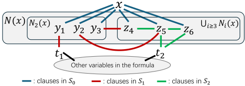
- S0: the set of clauses that contain variable x.
- S1: the set of clauses that contain variable(s) in N2(x) but not contain variable x.
- S2: the set of clauses that contain variable(s) in Ni(x), where i ≥ 3, but not contain any variable in N2(x)∪{x}.
By definition, S0, S1, S2 are pairwise disjoint. The primal graph of F shown in Figure 1 provides a useful perspective for understanding these notations and the subsequent proofs.
We plan to analyze the bounds for ∆t, ∆f , and ∆t +∆f by considering whether a clause in S0 ∪ S1 ∪ S2 would be removed after we assign a value to variable x (i.e., whether a clause would appear in R(F [x = 0]) or R(F [x = 0])).
Claim 1 (♣). All clauses in S0 and S1 would not appear in both R(F [x = 0]) and R(F [x = 1]).
By claim 1, we have ∆t ≥ |S0| + |S1| and ∆f ≥ |S0| + |S1|. Since |S0| = d (by definition) and |S1| = |N2(x)| (by Lemma 7), it holds that ∆t,∆f ≥ d + |N2(x)|.
Next, we consider the clauses in S2. Let D be a clause that contains variable x and a variable z ∈ Ni(x) where i ≥ 3. Assigning either x = 0 or x = 1 would make D become a 1clause that only contains variable z. When clause D becomes such 1-clause, R-Rule 4 would be applied to assign a value to z, and then remove all clauses containing z according to Lemma 8. Thus, for a clause in S2, it would not appear in at least one of R(F[x = 0]) and R(F[x = 1]). Together with previous analyses on S0 and S1, we have
To accurately characterize S2 (and |S2|), we need some additional notations. For a variable y ∈ N(x), we define P(y) := N(y)∩N(x) andQ(y) := N(y)\(N(x)∪{x}). For instance, in the example shown in Figure 1, we have P (z5) = {y2, z4, z6} and Q(z5) = {t2}. For each i ≥ 2 we define pi := ∑y∈Ni(x) |P(y)| and qi := ∑y∈Ni(x) |Q(y)|.
Claim 2 (♣). For all i ≥ 2, we have pi+qi = (i-1)|Ni(x)|.
We write p≥3 := ∑i≥3 pi and q≥3 := ∑i≥3 qi for brevity. The size of S2 is given in the following claim.
Claim 3 (♣). It holds that
By putting (2) into (1) and writing β := (p≥3 - p2) + 2(p2 + q2) + 2q≥3 for convenience, we have
Claim 4 (♣). It holds that
With (3), the lemma directly follows from Claim 4.
With Lemma 9 in hand, we proceed to determine the branching vectors of our branching operations.
Lemma 10 (♣). In Alg2CNF, the branching operation in Line 6 generates a branching vector not worse than (5, 11).
Lemma 11. In Alg2CNF, the branching operation in Line 8 generates a branching vector not worse than (4, 11).
Proof. In this branching operation, we branch on a 4-variable x with |N4(x)| ≥ 3. Note that in this step we have deg(F) = 4. By Lemma 9 with d = 4, we have ∆t, ∆f ≥ d = 4 and
By Lemma 1, the branching vector generated by this step is not worse than (4, 11).
Next, we analyze the phase three (Lines 10-11).
Lemma 12. Phase three (lines 10-11) of Alg2CNF can be excuted in O∗ (1.1082m) time.
Proof. When the algorithm reaches Line 10, the fomrula F is a reduced 2-CNF formula with d(F) ≤ 4 such that for every 4-variable x, |N4(x)| ≤ 2.
Let n := n(F), m := m(F), and ni (resp., n≥i) be the number of variables with degree i (resp., with degree ≥ i) in F , where i ∈ Z. Consider the primal graph G(F) of formula F. Note that n is also the number of vertices in G(F), and ni (resp., n≥i) is also the number of vertices with degree i in G(F). By Lemma 6, we have n1 = 0. Since d(F) ≤ 4, we have n≥5 = 0 and
By rearranging the above equation, we get
Let V4 be the set of 4-variables in the formula. The number of clauses that contain two 4-variables is 1 2 ∑x∈V4 |N4(x)|, and the number of clauses that contain at most one 4-variable is at least ∑x∈V4 (4 - |N4(x)|). Thus, we have
which means n4 ≤ m/3. By putting this into (4), we have
Let ϵ be a small constant (say 10-9 ) and nϵ be the corresponding integer (which is also a constant) in Theorem 1. Let n := n(F) and m := m(F). If n ≤ nϵ, we invoke algorithm Brute to solve the problem in constant time. Otherwise, if n > nϵ, we can apply Theorem 1 and get
Moreover, by Theorem 1, a path decomposition of G(F ) with width at most (4/27 + ϵ) m can be constructed in polynomial time. Then, we can apply Theorem 2 to solve the problem in time O∗ (2(4/27+ϵ)m) ⊆ O∗ (1.1082m).
Now we are ready to conclude a running-time bound of Algorithm Alg2CNF. By Lemma 10 and Lemma 11, branching operations in Line 6 and Line 8 generate a branching vector not worse than (5, 11) and (4, 11), respectively. By Lemma 12, phase three (Lines 10 and 11) takes O∗ (1.1082m) time. Since τ(5, 11) < 1.0956 and τ(4, 11) < 1.1058, we have the following result.
Theorem 4. Algorithm Alg2CNF solves WMC on 2-CNF formulas in O∗ (1.1082m) time, where m is the number of clauses in the input formula.
5 The Algorithm forWeighted #3-SAT
Our algorithm for WMC on 3-CNF formulas is called Alg3CNF and presented in Algorithm 2. The first phase is also to apply reduction rules to get a reduced instance. Note that by Lemma 3, a reduced formula is still a 3-CNF. The second phase is to branch on all 3+-variables. When the maximum degree of the formula is at most 2, we compute a path decomposition of the dual graph of the formula and then invoke the algorithm AlgDualPw to solve the problem.
5.1 The Measure
The analysis of the algorithm is different from that of the algorithm for #2-SAT. In this algorithm, it may not be effective to use m(F) as the measure in the analysis since we can not
Algorithm 2 Alg3CNF(F, w, W )
Input: 3-CNF formula F , weight function w, and integer W. Output: The weighted model count W · WMC(F, w).
- 1: Apply reduction rules exhaustively to reduce F and update w and W accordingly.
- 2: if F is empty then returnW.
- 3: if F contains empty clause then return 0.
- 4: if there is a d-variable x in F with d ≥ 3 then
- 5: Branch on x.
- 6: else
- 7: P ←path decomposition of Gd (F) via Theorem 1.
- 8: Wpw ←AlgDualPw(F,w, P);
- 9: return W · Wpw
guarantee this measure always decreases in all our steps. For example, a variable x may only appear as a positive literal in some 3-clauses. After assigning x = 0, it is possible that no reduction rule is applicable and no clause is removed (i.e., m(F) = m(R(F[x = 0]))). One of our strategies is to use the following combinatorial measure to analyze the algorithm
where mi(F)(i ∈ {2, 3}) is the number of i-clauses in formula F and 0 < α < 1 is a tunable parameter. Note that m(F) = m3(F) +m2(F) since there is no 1-clause in a reduced formula by Lemma 4 (we can simply assume that the initial input formula is reduced). Thus, µ(F) ≤ m(F). It can be verified that all the reduction rules would not increase µ(F) for any 0 < α < 1. If we can get a running time bound of O∗ (cµ(F) ), with a real number c > 1, we immediately get a running time bound of O∗ (cm(F ) ). We will first analyze the algorithm and obtain the branching vectors related to α, and then set the value of α to minimize the largest factor.
5.2 The Analysis
We first analyze lower bounds for the decrease of the measure µ(F) in a branching operation.
Lemma 13. Let F be a reduced 3-CNF formula, x be a variable in F, and ck(k ∈ {2, 3}) be the number of k-clauses containing variable x. Let ∆t := µ(F) - µ(R(F[x = 1])) and ∆f := µ(F) -µ(R(F[x = 0])). It holds that
- ∆t,∆f ≥ c2 · α+ c3 · (1-α);
- ∆t +∆f ≥ c2 · 2α+ c3 · (2-α).
Proof. Let Sℓk , where k ∈ {2, 3} and ℓ ∈ {x, ¯x}, be the set of k-clauses that contain literal ℓ. By definition, we have ck = |Sx k | + |S ¯x k | for k ∈ {2, 3}.
Consider what happens after we assign x = 1. First, all clauses containing literal x (i.e., clauses in Sx 3 and Sx 2 ) are satisfied (and so removed). This decreases ∆t by at least |Sx 3 | + |Sx 2 | · α. Second, all 3-clauses that contain literal ¯x (i.e., clauses in S ¯x 3 ) become 2-clauses. This decreses ∆t by at least |S ¯x 3 | · (1-α). Third, all 2-clauses that contain literal ¯x (i.e., clauses in S ¯x 2 ) become 1-clauses, and then R-Rule 4 would be applied to remove these clauses. This decreases ∆t by at least |S ¯x 2 | · α. In summary, we have
Analogously, we have ∆f ≥ c2 · α + c3 · (1 - α) + |S ¯x 3 | · α. Thus, ∆t,∆f ≥ c2 · α+ c3 · (1 -α) and
This completes the proof.
Armed with Lemma 13, we can derive the branching vectors generated by phase two (Line 5) in the algorithm.
Lemma 14. In Alg3CNF, the branching operation in Line 5 generates a branching vector not worse than the worst one of the following branching vectors:
Proof. Let x be a d-variable with d ≥ 3. Let p := c2 · 2α + c3 · (2 - α) and q := c2 · α + c3 · (1 - α). By Lemma 13, we have ∆t + ∆f ≥ p and ∆t, ∆f ≥ q. With Lemma 1, we know that the branching vector is not worse than (q, p-q) = (c2 · α+ c3 · (1-α), c2 · α+ c3). It is evident that larger c2 and c3 result in superior branching vectors. Since c2 + c3 = d ≥ 3, it suffices to consider the case where c2 + c3 = 3. By enumerating all four possible configurations of c2 and c3, we obtain the results stated in the lemma.
Next, we analyze the time complexity of phase three (Lines 7 and 8) in the algorithm.
Lemma 15. Phase three (Lines 7-8) of Alg3CNF can be executed in O∗ (1.1225 µ(F) α ) time.
Proof. When the algorithm reaches Line 7, the branching operation is not applicable. Thus, at this point, the formula F is a reduced 3-CNF formula with deg(F ) ≤ 2.
Let m := m(F) and µ := µ(F). Consider the dual graph Gd (F) of formula F . The number of vertices in Gd (F) is m. Let C ∈ F be a clause in formula F. We have |C| ≤ 3. Since each variable in C has a degree of at most two, the number of clauses that share a common variable with C is at most |C| ≤ 3. That is, for any C ∈ F, we have |{D ∈ F | D ̸= C and var(C) ∩ var(D) ̸= ∅}| ≤ 3.
This means that in Gd (F), each vertex has a degree of at most three. Let ni(i ∈ Z) be the number of vertices with degree i in Gd (F). We have ni = 0 for i ≥ 4 and n3 ≤ m. Let ϵ be a small const (say 10-9 ) and mϵ be the corresponding integer (which is also a constant) in Theorem 1. If m ≤ mϵ, we invoke brute-force algorithm Brute to solve the problem in constant time. Otherwise, if m > mϵ, we can apply Theorem 1 and get
| Phases | Branching vectors | Factors / Base α = 0.6309297 |
|---|---|---|
| Phase two | (3, 3 - 3α) | 1.4423 |
| (2 + α, 2 - α) | 1.4324 | |
| (1 + 2α, 1 + α) | 1.4325 | |
| (3α, 3α) | 1.4423 | |
| Phase three | - | 1.1225 1α = 1.2011 |
Here, the last inequality follows from m ≤ 1α µ, which can be derived by the definition of m and µ. In addition, by Theorem 1, a path decomposition of Gd (F) with width at most (1/6+ ϵ) µα can be constructed in polynomial time. Then, we can apply Theorem 3 to solve the problem in time O∗ (2 (1/6+ϵ)µ α ) ⊆ O∗ (1.1225 µα ).
We are now poised to analyze the overall running time of Alg3CNF. The time complexity of phase two (by Lemma 14) and phase three (by Lemma 15) are summarized in Table 1. By setting α = 0.6309297, the largest factor in phase two is minimized to 1.4423, corresponding to the branching vectors (3, 3 - 3α) and (3α, 3α). The time complexity of phase three is O∗ (1.1225 µ(F ) α ) ⊆ O∗ (1.2011µ(F) ). With µ(F) ≤ m(F), we arrive at the following result.
Theorem 5. Algorithm Alg3CNF solves WMC on 3-CNF formulas in O∗ (1.4423m) time, where m is the number of clauses in the input formula.
6 Conclusion and Discussion
In this paper, we demonstrate that Weighted Model Counting (WMC) on 2-CNF and 3-CNF formulas can be solved in O∗ (1.1082m) and O∗ (1.4423m) time, respectively, achieving significant improvements over previous results. The trivial barrier of O∗ (2m) for WMC on general CNF formulas cannot be overcome unless SETH fails [Cygan et al., 2016]. It remains an open question whether a running time bound of O∗ (cm) with a constant c < 2 can be achieved for WMC on k-CNF formulas for any constant k.
Our algorithms first use branch-and-search to effectively eliminate certain problem structures (such as high-degree vertices). Once the remaining problem exhibits some favorable structural properties (such as having a small primal pathwidth or dual pathwidth), dynamic programming and other methods are employed to solve the problem. This approach may have potential for application in solving other problems. Furthermore, this method holds significant promise in the design of practical algorithms. In practical solving, tree decompositions have been employed in various model counters [Dudek et al., 2020; Hecher et al., 2020; Fichte et al., 2019; Korhonen and J¨arvisalo, 2021; Fichte et al., 2022; Fichte et al., 2023b]. Therefore, the practicality of this approach warrants further investigation and exploration.
Acknowledgements
The work is supported by the National Natural Science Foundation of China, under the grants 62372095, 62172077, and 62350710215.
@inproceedings{ijcai2025p297,
  title     = {New Algorithms for #2-SAT and #3-SAT},
  author    = {Peng, Junqiang and Sheng, Zimo and Xiao, Mingyu},
  booktitle = {Proceedings of the Thirty-Fourth International Joint Conference on
               Artificial Intelligence, {IJCAI-25}},
  publisher = {International Joint Conferences on Artificial Intelligence Organization},
  editor    = {James Kwok},
  pages     = {2666--2674},
  year      = {2025},
  month     = {8},
  note      = {Main Track},
  doi       = {10.24963/ijcai.2025/297},
  url       = {https://doi.org/10.24963/ijcai.2025/297},
}
TY - CPAPER TI - New Algorithms for #2-SAT and #3-SAT AU - Peng, Junqiang AU - Sheng, Zimo AU - Xiao, Mingyu T2 - Proceedings of the Thirty-Fourth International Joint Conference on Artificial Intelligence, IJCAI-25 PB - International Joint Conferences on Artificial Intelligence Organization PY - 2025 SP - 2666 EP - 2674 DO - 10.24963/ijcai.2025/297 UR - https://doi.org/10.24963/ijcai.2025/297 ER -Copied
Machine-readable versions of this paper, for tools and AI agents:





