
ABNet: Mitigating Sample Imbalance in Anomaly Detection Within Dynamic Graphs
Proceedings of the Thirty-Fourth International Joint Conference on Artificial Intelligence. Main Track. Pages 2910-2918.
https://doi.org/10.24963/ijcai.2025/324
Keywords
- Data Mining: DM: Class imbalance and unequal cost
- Data Mining: DM: Networks
- Data Mining: DM: Anomaly/outlier detection
Abstract
In dynamic graphs, detecting anomalous nodes faces challenges due to sample imbalance, stemming from the scarcity of anomalous samples and feature representation bias. Existing methods often use unsupervised or semi-supervised learning to extract anomalous samples from unlabeled data, but struggle to obtain enough anomalous instances due to their low occurrence. Moreover, GNN-based approaches often prioritize normal samples, neglecting rare anomalies. To address these issues, we propose the Anomaly Balance Network (ABNet), designed to alleviate sample imbalance and enhance anomaly detection. ABNet includes three key components: a feature extractor that compares node features across time points to avoid bias, an anomaly augmenter that amplifies anomaly details and generates diverse anomalous samples, and an anomaly detector using meta-learning to adapt to graph evolution. Experimental results show that ABNet outperforms existing methods on three real-world datasets, effectively addressing sample imbalance.
- [Bandyopadhyay et al., 2019] Sambaran Bandyopadhyay, N Lokesh, and M Narasimha Murty. Outlier aware network embedding for attributed networks. In Proceed- ings of the AAAI conference on artificial intelligence, volume 33, pages 12-19, 2019.
- [Bock and Weiß, 2019] Sebastian Bock and Martin Weiß. A proof of local convergence for the adam optimizer. In 2019 international joint conference on neural networks (IJCNN), pages 1-8. IEEE, 2019.
- [Breunig et al., 2000] Markus M. Breunig, Hans Peter Kriegel, Raymond T. Ng, and Jörg Sander. Lof: Identi- fying density-based local outliers. In Acm Sigmod Inter- national Conference on Management of Data, 2000.
- [Ding et al., 2021] Kaize Ding, Qinghai Zhou, Hanghang Tong, and Huan Liu. Few-shot network anomaly detec- tion via cross-network meta-learning. In Proceedings of the Web Conference 2021, WWW '21, page 2448-2456, New York, NY, USA, 2021. Association for Computing Machinery.
- [Edwards, 1991] Tim Edwards. Discrete wavelet transforms: Theory and implementation. Universidad de, 1991:28-35, 1991.
- [Hamilton et al., 2017] Will Hamilton, Zhitao Ying, and Jure Leskovec. Inductive representation learning on large graphs. Advances in neural information processing sys- tems, 30, 2017.
- [Hershey and Olsen, 2007] John R Hershey and Peder A Olsen. Approximating the kullback leibler divergence between gaussian mixture models. In 2007 IEEE In- ternational Conference on Acoustics, Speech and Signal Processing-ICASSP'07, volume 4, pages IV-317. IEEE, 2007.
- [Hong et al., 2024] Yifan Hong, Chuanqi Shi, Junyang Chen, Huan Wang, and Di Wang. Multitask asynchronous metalearning for few-shot anomalous node detection in dynamic networks. IEEE Transactions on Computational Social Systems, pages 1-12, 2024.
- [Kiranyaz et al., 2021] Serkan Kiranyaz, Onur Avci, Osama Abdeljaber, Turker Ince, Moncef Gabbouj, and Daniel J Inman. 1d convolutional neural networks and applica- tions: A survey. Mechanical systems and signal process- ing, 151:107398, 2021.
- [Kumar et al., 2019] Srijan Kumar, Xikun Zhang, and Jure Leskovec. Predicting dynamic embedding trajectory in temporal interaction networks. In Proceedings of the 25th ACM SIGKDD international conference on knowl- edge discovery & data mining, pages 1269-1278, 2019.
- [Liu et al., 2023] Yixin Liu, Shirui Pan, Yu Guang Wang, Fei Xiong, Liang Wang, Qingfeng Chen, and Vincent CS Lee. Anomaly detection in dynamic graphs via trans- former. IEEE Transactions on Knowledge and Data En- gineering, 35(12):12081-12094, 2023.
- [Qin et al., 2020] Qi Qin, Wenpeng Hu, and Bing Liu. Fea- ture projection for improved text classification. In Pro- ceedings of the 58th Annual Meeting of the Association for Computational Linguistics, pages 8161-8171, 2020.
- [Reddy et al., 2017] R Ravinder Reddy, Y Ramadevi, and K.V.N Sunitha. Enhanced anomaly detection using ensem- ble support vector machine. In 2017 International Con- ference on Big Data Analytics and Computational Intelli- gence (ICBDAC), pages 107-111, 2017.
- [Tian et al., 2023] Sheng Tian, Jihai Dong, Jintang Li, Wen- long Zhao, Xiaolong Xu, Bowen Song, Changhua Meng, Tianyi Zhang, Liang Chen, et al. Sad: Semi-supervised anomaly detection on dynamic graphs. arXiv preprint arXiv:2305.13573, 2023. IJCAI
- [van der Maaten and Hinton, 2008] Laurens van der Maaten and Geoffrey Hinton. Visualizing data using t-sne. Journal of Machine Learning Research, 9(11):2579 -2605, 2008.
- [Vilalta and Drissi, 2002] Ricardo Vilalta and Youssef Drissi. A perspective view and survey of meta-learning. Artificial intelligence review, 18:77-95, 2002.
- [Wang and Bovik, 2009] Zhou Wang and Alan C. Bovik. Mean squared error: Love it or leave it? a new look at signal fidelity measures. IEEE Signal Processing Maga- zine, 26(1):98-117, 2009.
- [Wang and Zhang, 2022] Xiyuan Wang and Muhan Zhang. How powerful are spectral graph neural networks. In Inter- national conference on machine learning, pages 23341- 23362. PMLR, 2022.
- [Wang et al., 2021] Huan Wang, Chunming Qiao, Xuan Guo, Lei Fang, Ying Sha, and Zhiguo Gong. Identifying and evaluating anomalous structural change-based nodes in generalized dynamic social networks. ACM Transac- tions on the Web, 15(4):1-22, 2021.
- [Wang et al., 2022] Huan Wang, Qing Gao, Hao Li, Hao Wang, Liping Yan, and Guanghua Liu. A structural evolution-based anomaly detection method for general- ized evolving social networks. The Computer Journal, 65(5):1189-1199, 2022.
- [Wang et al., 2023a] Huan Wang, Guoquan Liu, and Po Hu. Tdan: Transferable domain adversarial network for link prediction in heterogeneous social networks. ACM Trans- actions on Knowledge Discovery from Data, 18(1):1-22, 2023.
- [Wang et al., 2023b] Huan Wang, Ruigang Liu, Chuanqi Shi, Junyang Chen, Lei Fang, Shun Liu, and Zhiguo Gong. Resisting the edge-type disturbance for link prediction in heterogeneous networks. ACM Transactions on Knowl- edge Discovery from Data, 18(2):1-24, 2023.
- [Xu et al., 2020] Da Xu, Chuanwei Ruan, Evren Korpeoglu, Sushant Kumar, and Kannan Achan. Inductive repre- sentation learning on temporal graphs. arXiv preprint arXiv:2002.07962, 2020.
- [Yao et al., 2019] Liang Yao, Chengsheng Mao, and Yuan Luo. Graph convolutional networks for text classification. In Proceedings of the AAAI conference on artificial intel- ligence, volume 33, pages 7370-7377, 2019.
- [Zhou and Paffenroth, 2017] Chong Zhou and Randy C Paf- fenroth. Anomaly detection with robust deep autoen- coders. In Proceedings of the 23rd ACM SIGKDD in- ternational conference on knowledge discovery and data mining, pages 665-674, 2017.
References were extracted automatically from the PDF and may contain errors.
Full text extracted automatically from the PDF; figures, tables and equations may differ. The PDF is the version of record.
1 Introduction
Dynamic graphs are characterized by evolving nodes and edges, reflecting changes in structure over time. In realworld scenarios such as social networks [Wang et al., 2023a; Wang et al., 2023b] and financial systems, anomaly detection is particularly challenging due to severe sample imbalance-normal samples vastly outnumber anomalous ones [Hong et al., 2024]. While normal nodes exhibit expected behaviors, anomalous nodes display irregular actions that may indicate underlying problems. For instance, in a financial payment system (see Figure 1), most users (nodes) perform routine transactions (edges), but a small minority may engage in fraudulent activities like credit card theft, deviating from typical patterns. Detecting these rare anomalous users is difficult because their scarcity limits the availability of training examples, making it hard for traditional methods to learn distinguishing features of anomalies. Therefore, effectively addressing sample imbalance is crucial for advancing anomaly detection in dynamic graphs.
∗ corresponding author
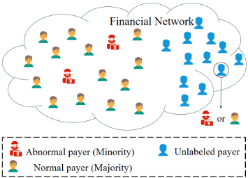
Existing approaches for anomaly detection in dynamic graphs often depend on mining anomalies from unlabeled data. Unsupervised methods, for example, identify anomalous nodes by measuring reconstruction errors in autoencoders [Zhou and Paffenroth, 2017] or by analyzing residuals from matrix decomposition techniques [Bandyopadhyay et al., 2019]. Semi-supervised strategies, such as SAD proposed by Tian et al. (2023), utilize large volumes of unlabeled data to detect anomalies in dynamic graph streams. Nevertheless, due to the inherent rarity of anomalies, unlabeled datasets frequently lack a sufficient number of anomalous samples, making it difficult to overcome the sample imbalance problem.
Addressing this issue requires tackling two main challenges. First, there is a need to reduce reliance on unlabeled data, which typically does not contain enough anomalous examples for robust model training. Since anomalous events are infrequent by nature, models that depend solely on unlabeled data struggle to learn diverse and representative anomaly patterns, limiting their ability to detect rare anomalies. Second, feature representation bias poses a significant obstacle. Graph Neural Network (GNN)-based methods often exhibit a bias toward the majority class (normal nodes) because they aggregate information from neighboring nodes. In imbalanced datasets, this aggregation process predominantly reflects the characteristics of normal nodes, causing the model to overlook the distinctive features of anomalous nodes.
To address these challenges, we propose the Anomaly Balance Network (ABNet), which is composed of three main modules: (i) Feature Extractor, (ii) Anomaly Augmenter, and (iii) Anomaly Detector. The Feature Extractor mitigates feature representation bias by emphasizing temporal variations in node features, rather than aggregating information solely from neighboring nodes. By capturing how a node's behavior changes over time, this component reduces the overwhelming influence of normal nodes and enhances the detection of anomalies. The Anomaly Augmenter tackles the scarcity of anomalous samples by generating synthetic anomalies through a combination of discrete wavelet transforms-which retain important feature details-and autoencoder-based perturbations. This strategy enriches the training set with diverse anomalous examples. The Anomaly Detector leverages a meta-learning framework that enables the model to adapt to evolving graph structures, improving its ability to identify new and emerging anomalies as the network changes. Experimental results on benchmark datasets demonstrate that ABNet surpasses existing methods, particularly by alleviating the sample imbalance problem and boosting anomaly detection performance.
We summarize the main contributions of this paper as follows:
- We introduce the Anomaly Balance Network (ABNet), which addresses feature representation bias by employing a feature extractor that emphasizes temporal variations in node behavior, rather than relying solely on information from neighboring nodes.
- We develop an anomaly augmentation method that generates synthetic anomalous samples by combining discrete wavelet transforms-preserving essential feature details-with autoencoder-based perturbations to enrich anomaly diversity.
- We design a meta-learning framework that enables the model to adapt to the evolving structure of dynamic graphs, improving its ability to detect newly emerging anomalies and generalize to unseen data.
- We conduct comprehensive experiments on real-world benchmark datasets, demonstrating that ABNet effectively detects anomalous nodes and mitigates sample imbalance. 1
2 RelatedWork
Anomalous node detection in dynamic graphs has emerged as a critical research area due to the complex and evolving nature of real-world networks [Wang et al., 2021]. Early approaches, such as the local density-based method proposed by [Breunig et al., 2000], identify anomalies by comparing a node's density to that of its neighbors. While effective in some settings, these methods often falter in the presence of severe class imbalance, as the scarcity of anomalies means their influence on local density is minimal, resulting in missed detections.
1 The code is available at an anonymous repository: https:// anonymous.4open.science/r/ABNet sample-F626.
| Symbol | Definition | Symbol | Definition |
|---|---|---|---|
| Gt | Dynamic graph at time t. | Vt | Nodes at time t. |
| Et | Edges at time t. | Ht | Node feature matrix at time t. |
| T | End time in the dynamic graph. | δ | Anomalous scores of nodes. |
| Φt | Feature difference in Gt. | ωt | Anomalous part of Φt. |
| W1,W2 | Weight matrices of the encoder. | W3,W4 | Weight matrices of the decoder. |
| St | Generated anomalous features. | ˆ Yi | Predicted label for node vi. |
| DWT | Discrete wavelet transform. | ˆ At | Normalized adjacency matrix of Gt |
| Yi | Ground truth label for node vi. | θ | Model parameters. |
| ϵt | random perturbations. | Dtask | Input of meta-tasks. |
| γ | Inner loop learning rate. | β | Outer loop learning rate. |
| A0 | Adjacency matrix of G0. | D0 | Degree matrix of G0. |
The development of dynamic graph learning has led to more sophisticated models. For example, TGAT [Xu et al., 2020] employs self-attention mechanisms and functional temporal encoding to capture temporal dependencies and dynamic node interactions. By embedding temporal information directly into the graph structure, TGAT can model evolving relationships. However, its performance is constrained by the need for large amounts of labeled data, making it less suitable for unsupervised or semi-supervised anomaly detection where labeled anomalies are rare.
To address the challenge of limited labeled data, Ding et al. (2021) introduced GDN, a graph neural network that leverages a small set of labeled anomalies to learn normal behavior patterns. GDN incorporates meta-learning, transferring knowledge from auxiliary networks to the main model, thereby enhancing adaptability to changing graph conditions and improving anomaly detection performance [Vilalta and Drissi, 2002]. This approach is particularly advantageous in highly dynamic environments where node behaviors shift rapidly.
Building on this, Tian et al. (2023) proposed SAD, a semisupervised anomaly detection framework that utilizes a memory bank to store the statistical distribution of normal samples. This memory provides valuable prior knowledge, aiding in the identification of anomalies. Nonetheless, SAD still faces significant challenges from class imbalance, as the overwhelming prevalence of normal data can obscure the detection of rare anomalous nodes.
Despite these advancements, a fundamental limitation persists: most existing methods depend heavily on unlabeled data. In imbalanced settings, the lack of sufficient anomalous samples within the unlabeled pool restricts the model's ability to learn diverse anomaly patterns, ultimately hindering performance in practical anomaly detection scenarios.
3 The Problem
Consider a dynamic graph G represented as a sequence of graph snapshots G = {G1,G2, . . . ,GT}, where each snapshot Gt = (Vt, Et) consists of a set of nodes Vt and edges Et at time t. Our objective is to identify anomalous nodes in the most recent snapshot GT .
Formally, we seek to compute the set AT = {⟨v, δ⟩ | v ∈ VT , δ ∈ [0, 1]}, where each node v ∈ VT is assigned an anomaly score δ that reflects the degree of abnormality, primarily based on its temporal feature evolution. Ideally, truly anomalous nodes would have δ = 1, while normal nodes would have δ = 0. The notations and symbols used throughout this work are summarized in Table 1.
4 ABNet
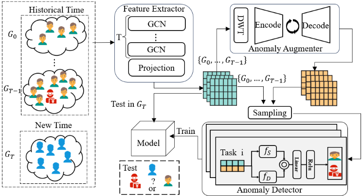
Overview. Figure 2 illustrates the overall architecture of ABNet, which is composed of three main modules: (i) Feature Extractor, (ii) Anomaly Augmenter, and (iii) Anomaly Detector.
The Feature Extractor is responsible for capturing and processing informative features from the dynamic graph, with a particular focus on the temporal evolution of node behaviors. The Anomaly Augmenter addresses the scarcity of anomalous samples by generating synthetic anomalies, thereby enriching the training set and enhancing the model's robustness. The Anomaly Detector leverages the features produced by the previous modules to identify nodes exhibiting abnormal patterns. The following sections provide detailed descriptions of each component.
4.1 Feature Extractor
The feature extractor in ABNet takes as input a sequence of normalized adjacency matrices { ˆ A0, ˆ A1, . . . , ˆ AT} and corresponding node feature matrices {H0,H1, . . . ,HT}. It employs multiple layers of Graph Convolutional Networks (GCNs) [Yao et al., 2019] to iteratively update node representations by aggregating information from each node's neighbors at every time step.
At the initial time step (t = 0), node features H0 are typically initialized randomly [Hamilton et al., 2017; Wang and Zhang, 2022]. The GCN then updates these features as follows:
where H′0 denotes the updated node features after applying the GCN at time step 0, W0 is the learnable weight matrix at time 0, and the normalized adjacency matrix at time step 0 is given by:
where D0 is the degree matrix of the adjacency matrix A0.
For each subsequent time step t > 0, the node features are updated by incorporating both the current graph structure Gt and the node features from the previous time step t - 1. Specifically, the features for nodes present in both Gt-1 and Gt are initialized using the updated features from the previous step:
where Nt-1 denotes the number of nodes at time t - 1, ensuring feature continuity across time. The GCN then refines these features for the current snapshot:
where H′ t is the updated node feature matrix at time t, ˆ At is the normalized adjacency matrix, and Wt is the learnable weight matrix for this step.
A common issue with GCNs is feature smoothing, which can mask anomalous behaviors by blending node features with those of their neighbors. To address this, we introduce a projection-based approach that emphasizes the temporal change in node features between consecutive time steps. The temporal feature difference, denoted as Φt, is computed as:
where proj(·, ·) denotes the projection operation, following the approach in [Qin et al., 2020]. In this context, Φt captures the temporal change in node features from time step t - 1 to t by projecting Ht onto Ht-1 and subtracting the aligned component. Specifically, let Ht-1,Ht ∈ RN×F be the node feature matrices at time steps t - 1 and t, where N is the number of nodes and F is the feature dimension. The term ⟨Ht-1,Ht⟩ denotes the inner product between the two feature matrices, and ∥Ht-1∥2 is the squared L2 norm of Ht-1. The expression Ht - ⟨Ht-1,Ht⟩ ∥Ht-1∥2 Ht-1 yields the component of Ht orthogonal to Ht-1, effectively quantifying the novel or changed information in the node features between consecutive time steps.
This projection-based difference, Φt = proj(Ht-1,Ht), thus isolates the temporal variation in node features, retaining the same shape as the original matrices (Φt ∈ RN×F ). By focusing on the orthogonal component, Φt highlights the degree and direction of feature evolution from t - 1 to t, providing a sensitive indicator for detecting abnormal or abrupt changes in node behavior over time.
4.2 Anomaly Augmenter
The anomaly augmenter in ABNet is designed to address the scarcity of anomalous samples by generating diverse synthetic anomalies, thereby enriching the training set and improving model robustness [Reddy et al., 2017]. Our augmenter is built upon an autoencoder framework, which consists of an encoder and a decoder, with additional mechanisms to preserve and enhance critical anomaly-related features.
Encoder. The encoder maps the input features of anomalous nodes into a compact latent representation. A key challenge in this process is the potential loss of fine-grained details that are crucial for distinguishing anomalies. To mitigate this, we integrate the Discrete Wavelet Transform (DWT) [Edwards, 1991] into the encoding pipeline. DWT decomposes the input into frequency components, allowing the model to retain high-frequency (detail-rich) information that may be indicative of anomalous behavior.
The input to the anomaly augmenter is the set of temporal feature differences for anomalous nodes, denoted as {ωt | t ∈ [0, T - 1]}, where each ωt is a subset of Φt corresponding to anomalous nodes at time t. The encoder processes each ωt as follows:
where W1 and W2 are learnable weight matrices, DWT(·) applies the discrete wavelet transform, and f(·) denotes a nonlinear transformation (e.g., a feedforward layer). This design ensures that the encoder captures both the global structure and the subtle, high-frequency variations present in anomalous node features.
Decoder. The decoder reconstructs the input from its latent representation and is responsible for generating synthetic anomalous samples. To achieve this, we inject random perturbations into the latent space by adding noise drawn from a standard normal distribution, ϵt ∼ N(0, 1), to the encoded vector z:
where W3 and W4 are the decoder's learnable weight matrices, g(·) denotes a nonlinear transformation (such as a feedforward layer), and St is the resulting synthetic anomalous feature. The addition of ϵt introduces stochasticity, enabling the generation of diverse anomalous samples that extend beyond the original data distribution. This process enhances the model's exposure to a broader range of anomaly patterns, thereby improving its ability to recognize and generalize to unseen anomalies.
To effectively balance the proportion of normal and anomalous samples in the training set, we repeat the perturbation and decoding process as necessary, generating a sufficient number of synthetic anomalous features to achieve the desired distribution for model training. This approach allows us to directly address sample imbalance by augmenting the minority class.
The autoencoder is optimized by minimizing the Mean Squared Error (MSE) loss [Wang and Bovik, 2009] between the original anomalous input ωt and its reconstructed output St:
where ωt denotes the original features of anomalous nodes at time step t, St is the corresponding generated anomalous feature, and T is the total number of time steps. We employ an enhanced version of the Adam optimizer [Bock and Weiß, 2019] to update the autoencoder parameters, ensuring stable and efficient convergence.
By generating diverse synthetic anomalies through random perturbations in the latent space, the anomaly augmenter enriches the training data and exposes the model to a broader spectrum of anomalous patterns. The integration of DWT in the encoder further preserves high-frequency, detail-rich features, enhancing the model's ability to detect subtle and complex anomalies.
4.3 Anomaly Detector
The anomaly detector in ABNet is responsible for identifying anomalous nodes by leveraging both temporal and augmented feature representations. To achieve robust detection, we construct meta-tasks by sampling node features at various time steps, enabling the model to learn from diverse temporal contexts and synthetic anomalies.
To effectively capture information at multiple levels of abstraction, we design a dual-channel architecture. One channel focuses on extracting deep, abstract features, while the other captures shallow, surface-level characteristics. This complementary structure ensures that both intricate patterns and immediate cues relevant to anomaly detection are utilized. Specifically, for each meta-task, the input Dtask is sampled from the union of synthetic anomalous features {S0, S1, . . . , ST-1} and temporal feature differences {Φ0,Φ1, . . . ,ΦT-1}. The combined feature representation is formulated as:
where α is a fusion coefficient balancing the contributions of the two channels. Here, fD denotes the deep feature extractor, implemented as a stack of five convolutional layers to capture
Algorithm 1 ABNet training process-flow.
Input:{ ˆ A0, ˆ A1, · · · , ˆ AT} and {H0,H1, · · · ,HT}. The learning rate for the inner loop γ. The learning rate for the outer loop β.
Extracting node features {Φ0,Φ1, · · · ,ΦT} by (1)-(5). Generate anomaly features {S0, S1, · · · , ST-1} by (7). Sampling meta-tasks from the set {S0, S1, · · · , ST-1} ∪ {Φ0,Φ1, · · · ,ΦT -1}.
for each training iteration do
for each meta-task input Dtask in meta-tasks do Compute dual-channel features by (9).
Compute Detection Loss by (10).
The parameter θ′i is updated by (11).
end for
The parameter θ′ is updated by (12).
end for
complex and abstract representations. fS denotes the shallow feature extractor, consisting of two convolutional layers to retain more immediate, low-level information. This dualchannel design enables the model to comprehensively represent node behaviors, as supported by prior work [Kiranyaz et al., 2021].
The anomaly detector outputs a prediction ˆ Yi(θ) for each node, where θ encompasses all learnable parameters. The ground truth anomaly label is denoted by Yi. We employ the binary cross-entropy loss to supervise training:
To enable rapid adaptation to evolving graph structures and distributions, we adopt a meta-learning framework with two nested optimization loops. The inner loop adapts the model to a specific meta-task, allowing it to quickly specialize to the sampled data. The outer loop aggregates experience across multiple meta-tasks, promoting generalization to new, unseen tasks. The parameter update in the inner loop is given by:
where θ is the initial parameter set, θ′i is the adapted parameter set for the i-th meta-task, Li(θ) is the task-specific loss, and γ is the inner loop learning rate.
In the outer loop, the model parameters are updated by aggregating gradients across all meta-tasks:
where θ′ is the updated parameter set, β is the outer loop learning rate, and Li(θ′i ) is the loss evaluated with the adapted parameters from the inner loop for each meta-task. This hierarchical optimization enables the model to learn both taskspecific and shared representations, enhancing its ability to detect anomalies in dynamic and imbalanced graph environments.
The complete training procedure for ABNet is detailed in Algorithm 1.
| Datasets | Nodes | Edges | Anomalies | Timespan |
|---|---|---|---|---|
| Wikipedia | 9,227 | 157,474 | 217 | 30 days |
| 10,984 | 672,447 | 366 | 30 days | |
| Mooc | 7,074 | 333,734 | 4,066 | 30 days |
Time Complexity. The overall time complexity of ABNet is determined by its three core modules: the feature extractor, the anomaly augmenter, and the anomaly detector. Specifically, the total complexity can be formulated as O(TLN 2 +KDM + IouterM ′ Iinner), where T is the number of time steps, L is the number of GCN layers, and N is the number of nodes (feature extractor); K is the number of encoder/decoder layers, D is the input feature dimension, and M is the number of training samples (anomaly augmenter); M ′ is the number of meta-tasks, and Iinner and Iouter are the numbers of inner and outer loop iterations in meta-learning (anomaly detector).
5 Experimentation
In this section, we present a comprehensive experimental study to assess the effectiveness of ABNet on standard benchmark datasets, comparing its performance with several stateof-the-art baseline methods. The following subsections provide detailed descriptions of the experimental setup, datasets, baselines, and evaluation protocols.
5.1 Experimental Settings
Datasets. We evaluate our approach on three real-world dynamic graph datasets [Kumar et al., 2019], summarized in Table 2:
Wikipedia: This data captures user edit events, with labels indicating if a user was blocked.
Reddit: This data captures user activity in subreddits, labeled by whether a user was banned.
Mooc: This data captures student interactions on online learning platforms, labeled by course dropout status.
Baseline Methods. We benchmark our framework against the following state-of-the-art baselines:
LOF [Breunig et al., 2000]: Identifies local outliers by comparing node density with neighbors.
GDN [Ding et al., 2021]: A few-shot anomaly detector using cross-network meta-learning with limited labeled anomalies.
TGAT [Xu et al., 2020]: Learns temporal graph representations via self-attention and time encoding.
SAD [Tian et al., 2023]: Semi-supervised method combining a time-aware memory bank and pseudo-label contrastive learning.
TADDY [Liu et al., 2023]: Transformer-based model capturing spatial and temporal information for anomaly detection in dynamic graphs.
Evaluation Metrics. We use the Area Under the Curve (AUC) as the primary metric to assess the performance of all methods. To ensure statistical reliability and reduce the influence of randomness, each experiment is independently repeated 20 times under the same settings.
Experimental Setup. We split each dataset into five temporal segments; the last segment is used for testing (75% for test, remainder for training/validation). Node features have dimension k = 128, with a batch size of 100. The anomaly augmenter uses a 5-layer autoencoder, and training employs an improved Adam optimizer [Bock and Weiß, 2019]. Experiments run on an Intel Xeon Gold 6132 CPU, 64GB RAM, and NVIDIA A100 GPU, with results averaged over 20 runs. We also conduct ablation, parameter sensitivity, clustering, and heatmap analyses.
5.2 Performance Comparison
Table 3 reports the AUC scores for all compared methods on the Wikipedia, Reddit, and Mooc datasets. ABNet achieves the highest AUCs across all datasets-92.21% on Wikipedia, 75.78% on Reddit, and 75.34% on Mooc-demonstrating strong adaptability to dynamic graph environments and resilience to class imbalance.
Among the baselines, LOF yields the lowest performance, with AUCs of 76.41% on Wikipedia and 54.41% on Mooc, indicating its limited capacity to handle evolving network structures. TGAT and GDN show moderate but inconsistent results: TGAT achieves 79.13% on Wikipedia, 67.06% on Reddit, and 66.88% on Mooc, while GDN attains 85.12% on Wikipedia but drops to 67.82% and 66.21% on Reddit and Mooc, respectively. The performance of GDN is likely hindered by insufficient anomaly diversity. SAD outperforms LOF and GDN on Mooc with an AUC of 69.44%, but its dependence on a small set of labeled anomalies limits its effectiveness. TADDY, which uses subgraph sampling, achieves 68.47% on Mooc; however, the use of duplicate samples may reduce the diversity of learned features.
Overall, ABNet consistently outperforms the baselines by combining meta-learning and data augmentation, which together improve anomaly diversity and enable the model to better capture dynamic changes in the graph.
5.3 Ablation Experiments
To assess the impact of each major component in ABNet, we conduct a series of ablation experiments, each removing or altering a specific module:
Without High-Frequency Feature Extraction (-E). Here, we exclude the high-frequency feature extraction from the anomaly augmenter. This leads to a clear reduction in performance, indicating that high-frequency features are essential for emphasizing fine-grained anomalies. Their absence makes it more difficult for the model to distinguish subtle abnormal patterns from normal behavior.
Without Dual-Channel Structure (-D). In this setting, we remove the dual-channel structure from the anomaly detector. The resulting performance drop suggests that the dualchannel design, which enables parallel processing of different data aspects, is important for learning richer and more diverse representations. Its removal reduces the model's robustness and accuracy in detecting anomalies.
Without Both High-Frequency Feature Extraction and Dual-Channel Structure (-D&E). When both highfrequency feature extraction and the dual-channel structure are removed, the model suffers the largest decrease in performance. As shown in Table 3, this combined ablation severely limits the model's ability to both amplify anomaly details and capture diverse information, highlighting the complementary roles of these two components.
Without Feature Projection (-P). In this experiment, we remove the feature projection module. Feature projection is responsible for capturing temporal changes in node features between consecutive time steps, which is critical for identifying subtle behavioral shifts [Wang et al., 2022]. Without it, the model's ability to track temporal dynamics is diminished, resulting in a noticeable decline in anomaly detection performance, as reflected in Table 3.
These ablation results collectively demonstrate that each component-high-frequency feature extraction, dual-channel structure, and feature projection-plays a vital role in the overall effectiveness of ABNet.
5.4 Parameter Sensitivity Analysis
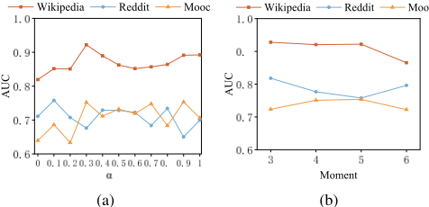
In this section, we perform a parameter sensitivity analysis to assess the stability and robustness of ABNet under varying parameter configurations. Specifically, we investigate how changes in the fusion weight α within the dual-channel structure and the number of time steps affect the model's performance.
Figure 3 presents the results of ABNet under different parameter settings. As illustrated in Figure 3a, the model's performance remains stable as the fusion weight α varies, indicating that ABNet effectively integrates both deep and shallow features and is resilient to changes in the weighting scheme.
We further examine the AUC scores obtained when training with different numbers of time steps, ranging from 3 to 6, across all datasets. As shown in Figure 3b, the model demonstrates only minor fluctuations in performance, underscoring its robustness to the choice of time window and its consistent effectiveness across datasets.
5.5 Visual Analyses
To gain deeper insights into the workings of ABNet and assess the impact of its feature extraction strategies, we present a set of visualization analyses. These visualizations demonstrate how the model responds to evolving network structures and differentiates between normal and anomalous nodes. The following subsections offer detailed visual evidence and interpretations drawn from these analyses.
| Method | LOF | TGAT | GDN | SAD | TADDY | ABNet | -E | -D | -D&E | -P |
|---|---|---|---|---|---|---|---|---|---|---|
| Wikipedia | 76.41 | 79.13 | 85.12 | 86.71 | 84.72 | 92.21 | 90.42 | 89.22 | 85.54 | 71.46 |
| 67.68 | 67.06 | 67.82 | 68.77 | 67.92 | 75.78 | 75.12 | 69.98 | 68.92 | 68.33 | |
| Mooc | 54.41 | 66.88 | 66.21 | 69.44 | 68.47 | 75.34 | 69.87 | 70.61 | 69.02 | 64.56 |
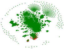
(b) ABNet's features with feature projection
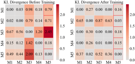
Figure 5: Heatmap of feature distributions across different time points before and after training on the Wikipedia dataset.
(a) Visualization of Node Features: Impact of Feature Projection.
We visualize the effect of feature projection on node representations to evaluate its role in anomaly detection.
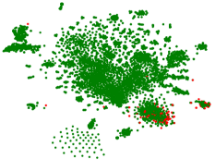
On the Reddit dataset, we use 2D t-SNE [van der Maaten and Hinton, 2008] to reduce node features from 128 to 2 dimensions. Figures 4a and 4b show node features from ABNet with and without orthogonal feature projection. Feature projection produces more distinct, compact clusters, making normal and anomalous nodes easier to separate. This indicates that projection improves the model's ability to capture temporal changes in node behavior.
By computing differences between node features across time steps, feature projection highlights temporal dynamics crucial for anomaly detection. Without this step, the model relies more on static features, which can cause overfitting and reduced sensitivity to evolving or subtle anomalies.
(b) Temporal KL Divergence Analysis. To assess our model's adaptation to temporal shifts in feature distributions, we compute the Kullback-Leibler (KL) divergence [Hershey and Olsen, 2007] between node features at different time points. Visualizing these divergences as heatmaps before and after training reveals how the model aligns feature distributions over time, which is important for robust anomaly detection in dynamic graphs.
Figure 5 shows KL divergence heatmaps for the Wikipedia dataset, with M denoting each time point. The fifth column, representing divergence between moment 5 and moments 14, initially shows high KL values before training, indicating large differences in feature distributions. After training, these values drop significantly, demonstrating that the model better aligns feature distributions across time. This reduction highlights improved adaptation to temporal distribution shifts and greater consistency in feature modeling.
5.6 Error analyses
We performed error analysis on a test set with both normal and anomalous nodes over multiple time steps to identify misclassification sources. Errors mainly fell into two categories:
- (a) False Positives, i.e., normal nodes flagged as anomalies. These include: (1) Temporal Fluctuations: Short-term behavioral changes in nodes, though normal, are sometimes misclassified as anomalies.
- Structural Changes: Network topology changes, like edge additions or removals, can be mistaken for anomalies.
- (b) False Negatives, i.e., missed anomalies. These include: (1) Subtle Anomalies: Some anomalies closely resemble normal behavior, making detection difficult.
- Anomaly Blending: Anomalies that overlap with broader network changes are less distinct and may be missed.
Most errors were false positives, often due to the network's dynamic nature-normal nodes sometimes show unusual behavior that the model flags as anomalous. False negatives were less frequent and usually occurred when anomalies mimicked normal patterns or were masked by network changes.
6 Conclusion
We proposed the Anomaly Balance Network (ABNet), a framework addressing sample imbalance in anomalous node detection for dynamic networks. Experiments on three realworld datasets show that ABNet outperforms state-of-the-art methods and mitigates sample imbalance. Future work will focus on improving anomaly augmentation and exploring dynamic network evolution to further enhance adaptability and robustness.
Acknowledgments
This work was supported by Project of the National Key R&D Program of China (2023YFD2400501) and the funding BAS/1/1689-01-01, URF/1/4663-01-01, REI/1/5232-0101, REI/1/5332-01-01, and URF/1/5508-01-01 from KAUST, and funding from KAUST - Center of Excellence for Generative AI, under award number 5940, Stable Support Project of Shenzhen (20231120161634002), Shenzhen Science and Technology Program (JCYJ20240813141417023), Natural Science Foundation of Guangdong Province of China (2025A1515010233), Guangdong Provincial Department of Education (2024KTSCX060), Tencent "Rhinoceros Birds" - Scientific Research Foundation for Young Teachers of Shenzhen University.
Contribution Statement
Yifan Hong and Muhammad Asif Ali are Co-first authors.
@inproceedings{ijcai2025p324,
  title     = {ABNet: Mitigating Sample Imbalance in Anomaly Detection Within Dynamic Graphs},
  author    = {Hong, Yifan and Ali, Muhammad Asif and Wang, Huan and Chen, Junyang and Wang, Di},
  booktitle = {Proceedings of the Thirty-Fourth International Joint Conference on
               Artificial Intelligence, {IJCAI-25}},
  publisher = {International Joint Conferences on Artificial Intelligence Organization},
  editor    = {James Kwok},
  pages     = {2910--2918},
  year      = {2025},
  month     = {8},
  note      = {Main Track},
  doi       = {10.24963/ijcai.2025/324},
  url       = {https://doi.org/10.24963/ijcai.2025/324},
}
TY - CPAPER TI - ABNet: Mitigating Sample Imbalance in Anomaly Detection Within Dynamic Graphs AU - Hong, Yifan AU - Ali, Muhammad Asif AU - Wang, Huan AU - Chen, Junyang AU - Wang, Di T2 - Proceedings of the Thirty-Fourth International Joint Conference on Artificial Intelligence, IJCAI-25 PB - International Joint Conferences on Artificial Intelligence Organization PY - 2025 SP - 2910 EP - 2918 DO - 10.24963/ijcai.2025/324 UR - https://doi.org/10.24963/ijcai.2025/324 ER -Copied
Machine-readable versions of this paper, for tools and AI agents:





