
OS-GCL: A One-Shot Learner in Graph Contrastive Learning
Proceedings of the Thirty-Fourth International Joint Conference on Artificial Intelligence. Main Track. Pages 2964-2972.
https://doi.org/10.24963/ijcai.2025/330
Keywords
- Data Mining: DM: Mining graphs
Abstract
Graph contrastive learning (GCL) enhances the self-supervised learning capacity for graph representation learning. Nevertheless, the previous research has neglected to consider one fundamental nature of GCL -- graph contrastive learning operates as a one-shot learner, guided by the widely utilized noise contrastive estimation (e.g., the InfoNCE loss). Theoretically, to initially investigate the factors that contribute to the one-shot learner essence, we analyze the InfoNCE-based objective and derive its equivalent form of the softmax-based cross-entropy function. It is concluded that the InfoNCE-based GCL is determined to be a (2n-1)-way 1-shot classifier (n is the number of nodes). In this particular context, each sample is indicative of a unique ideational class, and each class has only one sample. Consequently, the one-shot learning nature of GCL leads to the issue of the limited self-supervised signal. To further address the above issue, we propose a One-Shot Learner in Graph Contrastive Learning (OS-GCL). Firstly, we estimate the potential probability distributions of the deterministic node features and discrete graph topology. Secondly, we develop a probabilistic message-passing mechanism to propagate probability (of feature) on probability (of topology). Thirdly, we propose the ProbNCE loss functions to contrast distributions. Extensive experimental results demonstrate the superiority of OS-GCL. To the best of our knowledge, this is the first study to examine the one-shot learning essence and the limited self-supervised signal issue of GCL.
- [Chen et al., 2020] Ting Chen, Simon Kornblith, Mohammad Norouzi, and Geoffrey Hinton. A simple framework for contrastive learning of visual representations. In Interna- tional Conference on Machine Learning, pages 1597-1607, 2020.
- [Chuang et al., 2020] Ching-Yao Chuang, Joshua Robinson, Yen-Chen Lin, Antonio Torralba, and Stefanie Jegelka. De- biased contrastive learning. Advances in Neural Informa- tion Processing Systems, 33:8765-8775, 2020.
- [Hasanzadeh et al., 2021] Arman Hasanzadeh, Mo- hammadreza Armandpour, Ehsan Hajiramezanali, Mingyuan Zhou, Nick Duffield, and Krishna Narayanan. Bayesian graph contrastive learning. arXiv preprint arXiv:2112.07823, 2021.
- [Hassani and Khasahmadi, 2020] Kaveh Hassani and Amir Hosein Khasahmadi. Contrastive multi-view repre- sentation learning on graphs. In International Conference on Machine Learning, pages 4116-4126, 2020.
- [He et al., 2020] Kaiming He, Haoqi Fan, Yuxin Wu, Saining Xie, and Ross Girshick. Momentum contrast for unsuper- vised visual representation learning. In Computer Vision and Pattern Recognition, pages 9729-9738, 2020.
- [Hu et al., 2020] Weihua Hu, Matthias Fey, Marinka Zitnik, Yuxiao Dong, Hongyu Ren, Bowen Liu, Michele Catasta, and Jure Leskovec. Open graph benchmark: Datasets for machine learning on graphs. Advances in neural informa- tion processing systems, 33:22118-22133, 2020.
- [Jaiswal et al., 2020] Ashish Jaiswal, Ashwin Ramesh Babu, Mohammad Zaki Zadeh, Debapriya Banerjee, and Fillia Makedon. A survey on contrastive self-supervised learning. Technologies, 9(1):2, 2020.
- [Jang et al., 2017] Eric Jang, Shixiang Gu, and Ben Poole. Categorical reparameterization with gumbel-softmax. In In- ternational Conference on Learning Representations, 2017.
- [Ji et al., 2024] Cheng Ji, Zixuan Huang, Qingyun Sun, Hao Peng, Xingcheng Fu, Qian Li, and Jianxin Li. Regcl: Re- thinking message passing in graph contrastive learning. In Proceedings of the AAAI conference on artificial intelli- gence, pages 8544-8552, 2024.
- [Kipf and Welling, 2016] Thomas N Kipf and Max Welling. Variational graph auto-encoders. arXiv preprint arXiv:1611.07308, 2016.
- [Kipf and Welling, 2017] Thomas N. Kipf and Max Welling. Semi-supervised classification with graph convolutional networks. In International Conference on Learning Repre- sentations, 2017.
- [Liu et al., 2020] Zhao-Yang Liu, Shao-Yuan Li, Songcan Chen, Yao Hu, and Sheng-Jun Huang. Uncertainty aware graph gaussian process for semi-supervised learning. In Proceedings of the AAAI Conference on Artificial Intelli- gence, volume 34, pages 4957-4964, 2020.
- [Liu et al., 2021] Xiao Liu, Fanjin Zhang, Zhenyu Hou, Li Mian, Zhaoyu Wang, Jing Zhang, and Jie Tang. Self- supervised learning: Generative or contrastive. IEEE Trans- actions on Knowledge and Data Engineering, 35(1):857- 876, 2021.
- [Liu et al., 2022] Yixin Liu, Ming Jin, Shirui Pan, Chuan Zhou, Yu Zheng, Feng Xia, and S Yu Philip. Graph self-supervised learning: A survey. IEEE Transactions on Knowledge and Data Engineering, 35(6):5879-5900, 2022.
- [Logeswaran and Lee, 2018] Lajanugen Logeswaran and Honglak Lee. An efficient framework for learning sentence representations. In International Conference on Learning Representations, 2018.
- [Oord et al., 2018] Aaron van den Oord, Yazhe Li, and Oriol Vinyals. Representation learning with contrastive predictive coding. arXiv:1807.03748, 2018.
- [Perozzi et al., 2014] Bryan Perozzi, Rami Al-Rfou, and Steven Skiena. Deepwalk: Online learning of social rep- resentations. In Proceedings of the 20th ACM SIGKDD international conference on Knowledge discovery and data mining, pages 701-710, 2014.
- [Shchur et al., 2018] Oleksandr Shchur, Maximilian Mumme, Aleksandar Bojchevski, and Stephan Günnemann. Pit- falls of graph neural network evaluation. arXiv preprint arXiv:1811.05868, 2018.
- [Thakoor et al., 2021] Shantanu Thakoor, Corentin Tallec, Mohammad Gheshlaghi Azar, Rémi Munos, Petar Velick- ovic, and Michal Valko. Bootstrapped representation learn- ing on graphs. CoRR, abs/2102.06514, 2021.
- [Vallender, 1974] SS Vallender. Calculation of the wasser- stein distance between probability distributions on the line. Theory of Probability & Its Applications, 18(4):784-786, 1974.
- [Veličković et al., 2018] Petar Veličković, Guillem Cucurull, Arantxa Casanova, Adriana Romero, Pietro Liò, and Yoshua Bengio. Graph attention networks. In International Conference on Learning Representations, 2018.
- [Velickovic et al., 2019] Petar Velickovic, William Fedus, William L. Hamilton, Pietro Liò, Yoshua Bengio, and R. De- von Hjelm. Deep graph infomax. In International Confer- ence on Learning Representations, 2019.
- [Wang et al., 2022] Ruijia Wang, Xiao Wang, Chuan Shi, and Le Song. Uncovering the structural fairness in graph con- trastive learning. Advances in Neural Information Process- ing Systems, 35:32465-32473, 2022.
- [Wu et al., 2021] Lirong Wu, Haitao Lin, Cheng Tan, Zhangyang Gao, and Stan Z Li. Self-supervised learn- ing on graphs: Contrastive, generative, or predictive. IEEE Transactions on Knowledge and Data Engineering, 2021.
- [Xiao et al., 2023] Teng Xiao, Huaisheng Zhu, Zhengyu Chen, and Suhang Wang. Simple and asymmetric graph contrastive learning without augmentations. In Advances in Neural Information Processing Systems, 2023.
- [Xie et al., 2022] Yaochen Xie, Zhao Xu, Jingtun Zhang, Zhengyang Wang, and Shuiwang Ji. Self-supervised learn- ing of graph neural networks: A unified review. IEEE Transactions on Pattern Analysis and Machine Intelligence, 45(2):2412-2429, 2022.
- [Xu et al., 2021] Dongkuan Xu, Wei Cheng, Dongsheng Luo, Haifeng Chen, and Xiang Zhang. Infogcl: Information- aware graph contrastive learning. In Advances in Neural In- formation Processing Systems, pages 30414-30425, 2021.
- [Yeh et al., 2022] Chun-Hsiao Yeh, Cheng-Yao Hong, Yen- Chi Hsu, Tyng-Luh Liu, Yubei Chen, and Yann LeCun. Decoupled contrastive learning. In European Conference on Computer Vision, pages 668-684, 2022.
- [Zhang et al., 2021] Hengrui Zhang, Qitian Wu, Junchi Yan, David Wipf, and Philip S Yu. From canonical correlation analysis to self-supervised graph neural networks. Ad- vances in Neural Information Processing Systems, 34:76- 89, 2021.
- [Zhang et al., 2023] Yifei Zhang, Hao Zhu, Zixing Song, Pi- otr Koniusz, and Irwin King. Spectral feature augmentation for graph contrastive learning and beyond. In Proceed- ings of the AAAI Conference on Artificial Intelligence, vol- ume 37, pages 11289-11297, 2023.
- [Zhu et al., 2020] Yanqiao Zhu, Yichen Xu, Feng Yu, Qiang Liu, Shu Wu, and Liang Wang. Deep graph contrastive representation learning. arXiv preprint arXiv:2006.04131, 2020.
- [Zhu et al., 2021] Yanqiao Zhu, Yichen Xu, Feng Yu, Qiang Liu, Shu Wu, and Liang Wang. Graph contrastive learning with adaptive augmentation. In Proceedings of the Web Conference, pages 2069-2080, 2021.
References were extracted automatically from the PDF and may contain errors.
Full text extracted automatically from the PDF; figures, tables and equations may differ. The PDF is the version of record.
1 Introduction
Graph Contrastive Learning (GCL) has garnered significant research attention [Jaiswal et al., 2020; Liu et al., 2021], drawing inspiration from contrastive learning in computer vision [He et al., 2020; Chen et al., 2020; Chuang et al., 2020; Yeh et al., 2022] and natural language processing [Logeswaran and Lee, 2018; Oord et al., 2018]. GCL aims to acquire the representations of graph data without relying on labeled information and has demonstrated its superior effectiveness [Wu et al., 2021; Zhu et al., 2021; Xie et al., 2022; Liu et al., 2022; Ji et al., 2024]. The majority of GCL methods, which are based on the noise contrastive estimation (NCE) principle, typically contrast each sample with the others to detect differences, considering the augmented sample as a positive instance and all others as negatives [Velickovic et al., 2019; Hassani and Khasahmadi, 2020; Zhu et al., 2020]. Nevertheless, the principle of GCL is identified as a one-shot learning behavior in this paper and consequently introduces limited self-supervised signal challenges to GCL.
∗Corresponding Author.
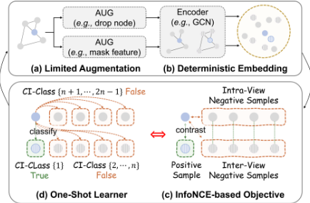
An overlooked fundamental nature of GCL. Upon closer examination of the optimization process of NCE-based graph contrastive learning (e.g., InfoNCE [Oord et al., 2018]), it becomes evident that GCL is essentially a (2n-1)-way 1-shot learner (n is the number of nodes). As illustrated in Figure 1, all other nodes are considered as classes (referred to as the "contrastive ideational class, CI-class" in this paper), while the target node is the sole sample in its class (i.e., the class represented by the positive sample). Consequently, there are 2n-1 CI-classes, with each class containing only one sample during training. It is important to note that the aforementioned 2n-1 CI-classes represent the ideational classes within the scope of GCL's objective, rather than the classes involved in downstream tasks, given the absence of label information during the training phase of self-supervised GCL. That is, GCL methods strive to be a theoretically one-shot learner. However, previous studies often overlook the aforementioned fact, leading to reduced effectiveness as a result of the following limited self-supervised signal challenges.
Given that there is only one sample in each CI-class, the deterministic feature/embedding in latent space is unable to accurately reflect the potential data distribution of the corresponding CI-class, that is, limited self-supervised signal problem. (1) Limited sample and supervision for each CI-class. GCL functions as a one-shot learner, with only one sample available in each CI-class. Previous studies have incorporated samples as a deterministic vector [Hassani and Khasahmadi, 2020; Zhu et al., 2020], leading to limitations in accurately estimating the feature distribution of each CI-class. The data augmentation technique utilized in GCL may offer an alternative approach; however, the limited number of random augmentations is insufficient to estimate the underlying probability distributions in one-shot classification. (2) Hard connection between different CI-classes. Different from contrastive learning in other domains, GCL typically utilizes graph neural networks (GNNs) to acquire the representations, following the message-passing schema [Kipf and Welling, 2017]. As the input topology is just one of the observable/observed possibilities in the real world, the observed hard connection between CI-classes cannot represent the real relationship between the potentially similar classes. Hence, it is essential to assess the probability distribution of topology and leverage it to propagate information within a profound sub-structure.
To further investigate and solve the aforementioned challenges, a theoretical analysis is undertaken to examine the reasons behind GCL's status as a one-shot learner and to offer insights from the perspective of probability. Furthermore, we propose a One-Shot Learner in Graph Contrastive Learning (OS-GCL), leveraging graph probability distribution estimation to enhance GCL through the lens of one-shot learning. Specifically, OS-GCL estimates the probability distributions pertaining to both node features and graph topology using multidimensional Gaussian distribution and Bernoulli distribution. Then, we propose a probabilistic message passing to aggregate the probability distribution on the non-discretized structure. Finally, we design the ProbNCE loss to contrast the distributions of positive and estimated negative samples. The primary contributions are summarized as follows:
- We identify that InfoNCE-based GCL is a 1-shot learner from the perspective of objective. To the best of our knowledge, this is the first to study 1-shot learning nature of GCL.
- Building upon the theoretical findings, we propose OS-GCL, improving the efficacy of GCL through graph probability distribution estimation using Gaussian and Bernoulli distributions, probabilistic message passing, and ProbNCE loss contrasting probability distributions.
- Extensive experiments demonstrate the superiority of OSGCL against state-of-the-art baselines.
2 Theoretical Analysis
This section begins with an overview of graph contrastive learning, providing background information. We further identify that graph contrastive learning is essentially a form of one-shot learning.
2.1 GCL under InfoNCE Principle
Consider a graph G = {V, E} with n nodes, where the set of nodes V = {vi}ni=1 and the set of edges E ⊆ V × V. Let A ∈ {0, 1}n×n denote the adjacency matrix of G and let X ∈ Rn×d represent the initial feature of nodes, where d signifies the input dimension of the feature.
Given a graph G = {V, E}, graph contrastive learning initially acquires two distinct views, {G u , G v }, by employing two different data augmentation techniques tu, tv ∼ T . GCL subsequently learns the embeddings of individual nodes by employing a node encoder (e.g., a GCN [Kipf and Welling, 2017]) and feeding them into a noise contrastive estimation loss function (e.g., InfoNCE loss [Oord et al., 2018]):
where u, v are the embeddings of nodes in the two augmented views, f(·, ·) = exp(sim(·, ·)/τ), sim(ui, vi) = ui · vi/||ui|| · ||vi|| is the cosine similarity, and τ is the temperature hyperparameter.
Note that different from graph-level graph contrastive learning, which can alter the number of nodes (e.g., subgraph sampling), the data augmentation functions t ∼ T in node-level GCL primarily consist of V-invariant augmentation.
Definition 1 (V-Invariant Augmentation). Given a graph G = {V, E}, a V-invariant augmentation t : G(V, E) → G ′ (V ′ , E ′ ) preserves the identity of the nodes, i.e., vi=v′i , i∈ [1, n]. This means that it does not involve the deletion or addition of nodes but only modifies the features of the nodes and the edges connecting them. A V-invariant augmentation is a bijective function w.r.t., nodes.
The V-invariant augmentation is commonly utilized in node-level GCL due to the node-level nature of downstream tasks [Hassani and Khasahmadi, 2020; Zhu et al., 2020], which necessitates GCL models to acquire embeddings for all original nodes. The bijection property guarantees that the identification of nodes in the augmented view remains, thereby supporting the assertion of Proposition 1 in the next section.
2.2 GCL is a (2n-1)-Way 1-Shot Learner
Given the formulation of InfoNCE-based graph contrastive learning (i.e., Eq.(1)), we can conclude the Proposition 1 by reformulating Eq.(1) into the form of a one-shot classification. The proof can be found in Appendix C.1.
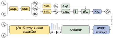
Proposition 1 (GCL is a (2n-1)-Way 1-Shot Learner). The InfoNCE-based graph contrastive learning method is a (2n-1)-way 1-shot classifier structured in the form of softmaxbased cross-entropy, given a graph G with n nodes, i.e., there are 2n-1 classes, each with only one sample. Let oi = ovii = sim(ui, vi)/τ be the predictive output and reformulate the InfoNCE into a form of softmax-based function:
where H(p(ui), q(ui)) is the cross-entropy between the predicted probability q(ui) based on softmax function and the true label p(ui).
Proposition 1 shows that the graph contrastive learning method based on InfoNCE is a softmax-based cross-entropy classifier, where each sample, except the target node ui, is considered a contrastive ideational class. From the proof, we can give the definition of contrastive ideational class.
Definition 2 (Contrastive Ideational Class, CI-class). The contrastive ideational class in graph contrastive learning is the virtual class in the perspective of optimizing InfoNCEbased GCL, represented by the other samples for each target sample, where the positive sample is the only true CI-class while the other negatives are the false CI-class.
As shown in Figure 2, decoupling the InfoNCE objective, the encoder along with the cosine similarity works as a classifier while the rest is a softmax-based cross-entory. In total, there are |V u | + |V v | - 1 = 2n - 1 CI-classes. Each node is assigned to a single class, as the augmentation functions do not alter the node from Definition 1, and each CI-class contains only one sample. That is, the InfoNCE-based GCL method can be described as a (2n-1)-way 1-shot classifier.
Remark 1. It is important to note that the aforementioned 2n-1 CI-classes represent the ideational classes within the scope of GCL's objective and are distinct from the actual classes in the dataset for downstream tasks. These ideational classes represent virtual categories from the perspective of optimization derived from the InfoNCE.
2.3 Rethinking GCL fromProbability Distribution
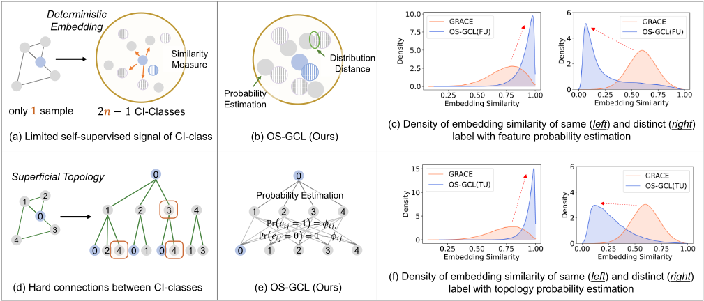
Drawing on the aforementioned theoretical findings, it has been observed that graph contrastive learning aims to acquire the representation of the node, which serves as the sole sample in its CI-class. The challenge of graph contrastive learning arises from the limited self-supervised signal. The scarcity of deterministic embeddings, such as only 1 in GCL, is insufficient to capture the potential distribution of each CI-class. Thus, estimating the probability distributions is crucial.
Specifically, as shown in Figure 3, (a) the limited selfsupervised signal is attributed to having only 1 sample per CI-classes. The existing deterministic embedding cannot represent the feature distribution of each CI-class, leading to a hard classification decision. In contrast, (b) we aim to estimate the probability distribution for each CI-class, facilitating the differentiation of distances. (c) Compared to the vanilla deterministic embedding approach, feature probability estimation can promote samples with the same label to be closer to each other; conversely, it can push different labels farther away. Similarly, (d) the hard connections between different CI-class can result in less accurate message-passing. (e) OS-GCL can propagate the probability of feature on the probability of topology, thus (f) improving the embedding affinity within the same label and enhancing the distinctiveness between different labels. Please refer to Appendix H.3 for more detailed experimental results about the embedding similarity.
3 Methodology
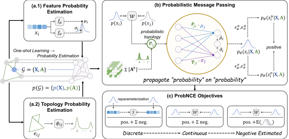
Considering that the principle of GCL ultimately involves a form of (2n - 1)-way 1-shot learning rooted in prior theoretical discoveries, We therefore propose a One-Shot Learner in Graph Contrastive Learning (OS-GCL), leveraging probability estimation to address the lower efficacy resulting from the limited training samples for each CI-class in the optimization.
3.1 Feature and Topology Probability Estimation
In order to ease the limited self-supervised signal in one-shot learning of GCL, we propose to estimate the potential feature and topology distribution from the limited training data provided for each positive sample (i.e., CI-classes).
Feature Probability Estimation. To estimate the feature probability distribution for each CI-class, it is necessary to identify an appropriate distribution that can accurately depict the potential distribution of samples for each class while being constrained to only utilizing the single provided sample (i.e., the target node i). As indicated in previous studies [Kipf and Welling, 2016], it is possible to utilize a Gaussian distribution N(µ, σ) to model the initial distribution of the data, with the input data being considered as samples drawn from this distribution. Therefore, we propose to learn the potential distributions p(xi) for each specified target node i ∈ V by employing the multidimensional Gaussian distribution:
where µi represents the estimated mean vector of the potential distribution that generates xi, and σi denotes the variance vector of the learned Gaussian distribution. The estimators fµ and fσ are single-layer linear, responsible for the mean and variance vectors.
Topology Probability Estimation. Unlike other forms of data (e.g., images/sentences), in addition to feature probability, graph data also includes the graph structure. The final embeddings incorporate topology features through the messagepassing of GNNs which utilize the edges to propagate the neighborhood information. Each edge eij in the graph topology can be interpreted as a complete probability (i.e., Aij = 1) of node i being connected to node j. However, the probabilities associated with each edge of 0/1 ∈ A are only reflected by one single glance (i.e., the 1st order proximity), yet the actual probabilities are concealed within the node feature and sub-structures. Instead of a deterministic value, a probability of whether linking is more consistent with the actual situation, particularly in a one-shot setting. Therefore, in order to fully capture the probability distribution of graph data, we also suggest employing the Bernoulli distribution to characterize the probability of the topology, representing each edge as an independent random variable from Bernoulli(·). Specifically, the probability distribution of topology for each edge eij can be estimated with the probability parameter ϕij ∈ [0, 1]:
where the probability parameter ϕij plays a crucial role in estimating the probability distribution of the topology. Specifically, the notation Bernoulli(ϕij) indicates that node i has a probability of ϕij of being connected to node j.
3.2 Probabilistic Message Passing: Probability Propagation on Probability
Furthermore, a novel graph encoder is developed to propagate the distribution information of nodes p(xi) = N(µi, σi) by means of the edge probabilities p(eij) = Bernoulli(ϕij).
Propagation Probability fromTopology Distribution. We propose a meticulously crafted learnable function that operates on both the node feature and sub-structures to derive the probability parameter ϕij . The distance between the feature distribution of node i (i.e., CI-class i) and node j (i.e., CIclass j) can directly indicate the probability of the edge eij. Nevertheless, different from the deterministic embeddings, the distance between two probability distributions is more challenging to compute compared to the Euclidean distance or cosine similarity used to measure the distance between deterministic embeddings. One potential approach involves directly utilizing the divergence value (e.g., KL-divergence or JS-divergence) to quantify the distance between distributions. However, the divergence does not function as a measurement of distance, as it does not adhere to all properties of distance (e.g., the symmetry or the triangle inequality). Moreover, when the distributions of two nodes do not or little overlap (e.g., negative samples), JS divergence is constant in this case, and the KL divergence becomes meaningless. Therefore, we propose to utilize the Wasserstein distance [Vallender, 1974] to achieve the above aims, quantifying the disparity between the feature distributions:
where Wij = W(p(xi)||p(xj)) and dij = ||µi -µj||2 . In addition to leveraging the Wasserstein distance of feature probability distribution, we further propose to learn the higherorder proximities in graph data. Specifically, we propose to use the higher-order transition probabilities A = ∑ki=1 Ai , where A denotes the adjacency matrix, and k represents the hyperparameter used to regulate the maximum order of the higher-order transition probabilities. A offers a purely structural approach to understanding the probability of linking. When combined with a decreasing function of the Wasserstein distance W(p(xi||xj)) (where a smaller Wasserstein distance indicates a higher feature correlation), it constitutes the function of the probability parameter:
where α represents the weight coefficient used to control the balance between feature distance and topology proximity, and σ(x) = exp(-x) is the activation function. Note that the higher-order transition probability A can be computed during the preprocessing of the dataset and does not need to be calculated at every iteration in the training process, thus not increasing the computational complexity. For further details, please refer to the experimental results of training time in Appendix H.2.
The final step to obtain the probabilistic topology Pij is to make it differentiable w.r.t. Bernoulli(ϕij), which is truthfully a binary specific case of categorical distribution. In this paper, we adopt the Gumbel-softmax [Jang et al., 2017] to estimate the non-differentiable probabilistic topology from the Bernoulli distribution. Please refer to Appendix C.2 for a detailed derivation. The final formulation of the probabilistic topology is:
where ϵij ∼ Uniform(0, 1) and τ1 represents the temperature. We filter out edges with smaller values. We use two encoders (i.e., mean encoder and variance encoder) to obtain the distribution of embedding pθ(zi | X, A) = N( ˆµi, ˆσi), which is based on the learned probabilistic topology. We next design a distribution perturbation mechanism to create augmented views of the embedding, rather than randomly augmenting the input data. More details can be found in Appendix E.
3.3 ProbNCE Loss
As for the objective functions, we design two different versions, discrete ProbNCE and continuous ProbNCE.
Discrete ProbNCE (ProbNCE-D). One can easily obtain two deterministic embeddings from the original embeddings pθ(zi |X,A) without introducing distribution perturbation. Then, reparameterization tricks [Kipf andWelling, 2016] can be used to generate the positive and negative samples. Then we can use the original InfoNCE loss in Eq.(1) as the objectives.
Continuous ProbNCE (ProbNCE-C). Beyond the discrete ProbNCE, we further propose the continuous ProbNCE function. Since the cosine similarity in the original InfoNCE is used to measure the distance between deterministic representations, we can use the Wasserstein distance to measure the difference between distributions, similar to Eq.(5) used in probabilistic message-passing and formulate it as follows:
Optimization with Negative Distribution Estimation. We can reformulate the InfoNCE loss as mathematical expectations:
where η = n - 1 in this paper, denoting the ratio of negative samples to the positive (i.e., 2η : 1). Then we can estimate the exceptions using the probability distribution of all negatives.
where pθ(zneg,u/v i |X,A) are the estimated negative distributions of target node i. Then the loss is formed as:
where pn,v i = pθ(zneg,v i |X,A) for simplicity. Please refer to the Appendix B.2 for the complexity analysis.
| Methods | Input | Cora | CiteSeer | PubMed | Photo | CS | Physics |
|---|---|---|---|---|---|---|---|
| Supervised GCN [Kipf andWelling, 2017] | X,A,Y | 82.5±0.4 | 71.2±0.3 | 79.2±0.3 | 92.4±0.2 | 93.0±0.3 | 95.7±0.2 |
| Supervised GAT [Veliˇckovi´c et al., 2018] | X,A,Y | 83.0±0.7 | 72.5±0.7 | 79.0±0.3 | 92.6±0.4 | 92.3±0.2 | 95.5±0.2 |
| UaGGP [Liu et al., 2020] | X,A,Y | 82.7 | 70.7 | 76.7 | - | - | - |
| Raw Features | X | 47.9±0.4 | 49.3±0.2 | 69.1±0.3 | 78.5±0.0 | 90.4±0.0 | 93.6±0.0 |
| Linear CCA | X | 58.9±1.5 | 27.5±1.3 | 75.8±0.4 | 86.9±0.7 | 93.1±0.2 | 95.0±0.2 |
| DeepWalk [Perozzi et al., 2014] | A | 70.7±0.6 | 51.4±0.5 | 74.3±0.9 | 89.4±0.1 | 84.6±0.2 | 91.8±0.2 |
| VGAE [Kipf and Welling, 2016] | X,A | 71.5±0.4 | 65.8±0.4 | 72.1±0.5 | 91.6±0.1 | 90.0±0.7 | 94.9±0.1 |
| DGI [Velickovic et al., 2019] | X,A | 82.2±0.6 | 71.2±0.5 | 84.0±0.3 | 91.6±0.2 | 91.7±0.1 | 94.4±0.2 |
| GRACE [Zhu et al., 2020] | X,A | 81.5±0.3 | 71.6±0.2 | 80.5±0.3 | 92.2±0.2 | 92.8±0.1 | 95.0±0.1 |
| InfoGCL [Xu et al., 2021] | X,A | 83.5±0.3 | 73.5±0.4 | 79.1±0.2 | - | - | - |
| MVGRL [Hassani and Khasahmadi, 2020] | X,A | 83.1±0.1 | 73.3±0.3 | 80.2±0.1 | 91.7±0.1 | 92.3±0.1 | 95.3±0.1 |
| BGRL [Thakoor et al., 2021] | X,A | 81.7±0.5 | 72.1±0.5 | 80.2±0.4 | 92.6±0.3 | 93.0±0.2 | - |
| CCA-SSG [Zhang et al., 2021] | X,A | 83.6±0.3 | 72.7±0.4 | 80.9±0.2 | 93.2±0.1 | 93.1±0.2 | 95.3±0.1 |
| BGCL [Hasanzadeh et al., 2021] | X,A | 83.8±0.3 | 72.7±0.3 | - | 92.5±0.2 | - | - |
| SpCo [Zhang et al., 2023] | X,A | 82.3±0.4 | 70.9±0.2 | 81.3±0.4 | - | - | - |
| GRADE [Wang et al., 2022] | X,A | 83.3±0.5 | 68.2±0.6 | 81.5±0.5 | 92.6±0.3 | 93.2±0.3 | - |
| GraphACL [Xiao et al., 2023] | X,A | 84.2±0.3 | 73.6±0.2 | 82.2±0.1 | 93.3±0.1 | - | - |
| OS-GCL (Ours) | X,A | 84.7±0.5 | 74.1±0.6 | 84.3±0.2 | 92.8±0.3 | 93.4±0.4 | 95.8±0.1 |
comparison to the baselines that also enhance the loss function (e.g., CCA-SSG), OS-GCL continues to demonstrate superior performance, up to 3.4% improvement. Please refer to the ablation study in the following section for a more comprehensive analysis of each main component of OS-GCL. Furthermore, OS-GCL outperforms methods that focus on distribution estimation (e.g., BGCL) with an improvement up to 1.4%. This indicates that the proposed probabilistic message-passing and ProbNCE loss offer greater benefits to performance.
Large-Scale Dataset. We also evaluate OS-GCL on one large-scale graph dataset, ogbn-arXiv [Hu et al., 2020]. The proposed OS-GCL still achieves competitive performance on both the validation and test sets, showing the scalability of OS-GCL. Please refer to Appendix H.1 for more results.
4.3 Ablation Study
Effect of Probability Estimation. From Table 2, it is noticed that the performance decreases without probability estimation, which reflects that the probability learning of graph data can help GCL from its one-shot learning essence. Specifically, when removing feature probability estimations, the performance slightly decreases because this variant still suffers from the limited samples for each CI-class in the one-shot learning essence of GCL. Similarly, the topology probability estimation improves the effectiveness due to capturing the possibilities of node interactions.
Effect of ProbabilisticMessage-Passing. It is demonstrated that the proposed probabilistic message-passing is crucial to the performance of OS-GCL from Table 2. Note that the impact of topology proximity is very severe (even less than GRACE) since the structure information is important to the graph. Furthermore, the performance drops 2.4% after removing the higher order, and the distribution perturbation on the embedding is more suitable for the proposed OS-GCL framework than the random augmentation.
4 Experiments
4.1 Experimental Setup
Datasets. We evaluate OS-GCL 1 on seven node classification benchmarks: (1) Citation networks [Kipf and Welling, 2017]: Cora, CiteSeer, and PubMed. (2) Co-purchase networks [Shchur et al., 2018]: Amazon Photo. (3) Co-author networks [Shchur et al., 2018]: Coauthor CS and Coauthor Physics. (4) Large dataset [Hu et al., 2020]: ogbn-arXiv.
Baselines. We evaluate OS-GCL in comparison with the following baselines: GCN [Kipf and Welling, 2017], GAT [Veliˇckovi´c et al., 2018], UaGGP [Liu et al., 2020], DeepWalk [Perozzi et al., 2014], VGAE [Kipf and Welling, 2016], DGI [Velickovic et al., 2019], GRACE [Zhu et al., 2020], InfoGCL [Xu et al., 2021], MVGRL [Hassani and Khasahmadi, 2020], BGRL [Thakoor et al., 2021], SpCo [Zhang et al., 2023], CCA-SSG [Zhang et al., 2021], BGCL [Hasanzadeh et al., 2021], GRADE [Wang et al., 2022], and GraphACL [Xiao et al., 2023]. Details are listed in Appendix F.
4.2 Main Results
From Table 1, it is evident that OS-GCL outperforms the current state-of-the-art graph representation learning and graph contrastive learning. Compared to GRACE, which could be considered the foundation of our approach, the enhancement reaches up to 3.8%. In addition, when compared to the baselines employing robust data augmentation methods (e.g., GRADE), OS-GCL contains 2.1% improvements on average which are contributed to the incorporation of distribution estimation techniques, including the Gaussian and Bernoulli distributions, as well as distribution perturbation, all achieved without the necessity of random augmentations. In Effect of ProbNCE. In OS-GCL, we design three types of ProbNCE loss functions. Among them, the continuous version with negative estimation beats the others. This suggests that sampling a deterministic one from the probabilistic embedding is not helpful and directly contrasting the distance contains high efficacy. Furthermore, without the negative estimation, the performance also decreases because contrasting a large number of negative distributions may cause the opposite effect (e.g., model confusion). In addition, negative estimation also improves the efficiency of the model.
1 The code and appendix are available at https://github.com/ RingBDStack/OS-GCL.
| Variants | Cora | CiteSeer | PubMed | Photo | CS | Physics |
|---|---|---|---|---|---|---|
| OS-GCL (Ours) | 84.7±0.5 | 74.1±0.6 | 84.3±0.2 | 92.8±0.3 | 93.4±0.4 | 95.8±0.1 |
| w/o Feature probability estimation | 84.0±0.2 | 72.4±0.3 | 82.9±0.1 | 92.3±0.5 | 92.9±0.2 | 95.5±0.1 |
| w/o Topology probability estimation | 83.2±0.4 | 71.2±0.6 | 83.2±0.2 | 92.3±0.3 | 93.0±0.1 | 95.4±0.2 |
| w/o probability estimation (Both) | 81.9±0.4 | 71.2±0.5 | 80.6±0.4 | 92.2±0.2 | 92.9±0.0 | 95.3±0.1 |
| w/o Feature in Probabilistic Message-Passing w/o Topology in Probabilistic Message-Passing | 83.0±0.5 | 72.6±0.5 | 83.2±0.1 | 91.9±0.4 | 93.0±0.1 | 95.4±0.2 |
| 77.5±0.5 | 60.5±0.9 | 77.2±0.2 | 88.4±0.4 | 90.6±0.2 | 95.3±0.1 | |
| w/o Higher Order in Probabilistic Message-Passing | 83.8±0.9 | 72.5±0.5 | 82.0±0.1 | 92.4±0.2 | 92.9±0.2 | 95.6±0.1 |
| w/o distribution perturbation | 81.9±0.5 | 72.2±0.5 | 81.2±0.2 | 91.5±0.4 | 92.5±0.2 | 95.3±0.2 |
| repl. KL Divergence | 84.4±0.1 | 73.2±0.2 | 83.1±0.3 | 90.8±0.4 | 92.9±0.2 | 95.4±0.1 |
| repl. JS Divergence | 83.1±0.1 | 72.9±0.3 | 84.0±0.2 | 90.1±0.2 | 92.8±0.3 | 95.3±0.3 |
| w/o ProbNCE-C | 83.3±0.6 | 72.2±0.5 | 83.7±0.1 | 92.2±0.3 | 92.8±0.1 | 95.3±0.1 |
| w/o Wassertein Distance in ProbNCE-C | 83.1±0.7 | 72.1±0.8 | 83.8±0.3 | 92.1±0.4 | 92.7±0.2 | 95.4±0.2 |
| w/o Negative Estimation in ProbNCE-C | 84.1±0.5 | 71.5±0.8 | 82.4±0.2 | 91.8±0.3 | 92.9±0.2 | 95.2±0.2 |
4.4 Hyperparameter Sensitivity
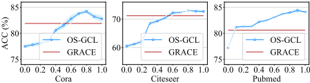
Feature-Topology Trade-Off Weight α. The proposed probabilistic message-passing is controlled by the featuretopology trade-off hyperparameter α in Eq.(6). From Figure 5, we found that only feature distance (i.e., α = 0) or only topology proximity (i.e., α = 1) cannot achieve the best performance. Furthermore, with less topology information (i.e., a small value of α), the efficacy drops severely, even worse than GRACE, demonstrating the importance of structural information for graph probability estimation.
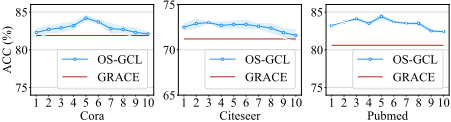
Number of Orders k. In Figure 6, it is noticed that a proper large value of k (3 ∼ 5 practically) is beneficial to the performance. That is, only the initial structure is not enough to learn the probability distribution of topology, yet a larger number of k may damage the effectiveness due to the over-smoothing.
4.5 Training Time Analysis
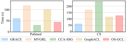
To investigate the runtime of OS-GCL, we provide the whole time cost of OS-GCL in Figure 7. We have the following observations: OS-GCL contains the competitive time cost, even compared to the vanilla GRACE. The proposed distribution perturbation in message-passing and negative estimation in ProbNCE loss makes a large contribution to the time cost reduction. The distribution perturbation avoids the double forward computational cost of GNNs. In addition, negative estimation in ProbNCE reduces the computation of negative scores. We evaluate the time cost of A in Appendix H.2 which is appropriate compared to the whole training.
5 Conclusion
In this paper, we point out a fundamental nature of graph contrastive learning that GCL is essentially a one-shot learner and thus faces the limited self-supervised signal issue. We further propose a one-shot learning in graph contrastive learning (OSGCL) leveraging the probability distribution estimation, probabilistic message passing, and ProbNCE loss. OS-GCL leverages the Gaussian distribution and Bernoulli distribution to learn the probability of feature and topology. The experimental results demonstrate the superior efficacy of OS-GCL.
Acknowledgments
We thank the anonymous reviewers for their insightful comments and suggestions. The corresponding author is Jianxin Li. The authors of this paper were supported by the NSFC through grant No.62225202 and No.62402054.
@inproceedings{ijcai2025p330,
  title     = {OS-GCL: A One-Shot Learner in Graph Contrastive Learning},
  author    = {Ji, Cheng and He, Chenrui and Li, Qian and Sun, Qingyun and Fu, Xingcheng and Li, Jianxin},
  booktitle = {Proceedings of the Thirty-Fourth International Joint Conference on
               Artificial Intelligence, {IJCAI-25}},
  publisher = {International Joint Conferences on Artificial Intelligence Organization},
  editor    = {James Kwok},
  pages     = {2964--2972},
  year      = {2025},
  month     = {8},
  note      = {Main Track},
  doi       = {10.24963/ijcai.2025/330},
  url       = {https://doi.org/10.24963/ijcai.2025/330},
}
TY - CPAPER TI - OS-GCL: A One-Shot Learner in Graph Contrastive Learning AU - Ji, Cheng AU - He, Chenrui AU - Li, Qian AU - Sun, Qingyun AU - Fu, Xingcheng AU - Li, Jianxin T2 - Proceedings of the Thirty-Fourth International Joint Conference on Artificial Intelligence, IJCAI-25 PB - International Joint Conferences on Artificial Intelligence Organization PY - 2025 SP - 2964 EP - 2972 DO - 10.24963/ijcai.2025/330 UR - https://doi.org/10.24963/ijcai.2025/330 ER -Copied
Machine-readable versions of this paper, for tools and AI agents:





