
HA-SCN: Learning Hierarchical Aligned Subtree Convolutional Networks for Graph Classification
Proceedings of the Thirty-Fourth International Joint Conference on Artificial Intelligence. Main Track. Pages 3245-3253.
https://doi.org/10.24963/ijcai.2025/361
Keywords
- Machine Learning: ML: Convolutional networks
- Data Mining: DM: Mining graphs
Abstract
In this paper, we propose a Hierarchical Aligned Subtree Convolutional Network (HA-SCN) for graph classification. Our idea is to transform graphs of arbitrary sizes into fixed-sized aligned graphs and construct a normalized K-layer m-ary subtree for each node in the aligned graphs. By sliding convolutional filters over the entire subtree at each node, we define a novel subtree convolution and pooling operation that hierarchically abstracts node-level information. We demonstrate that the proposed HA-SCN model not only realizes the convolution mechanism similar to the Convolutional Neural Networks (CNNs), which have the characteristics of weight sharing and fixed-sized receptive fields, but also effectively mitigates the over-squashing problem. Meanwhile, it establishes the correspondence information between nodes, alleviating the information loss issue. Experimental results on various benchmark graph datasets show that our approach achieves state-of-the-art performance in graph classification tasks.
- [Alon and Yahav, 2021] Uri Alon and Eran Yahav. On the Bottleneck of Graph Neural Networks and its Practical Im- plications. In Proceedings of ICLR, 2021.
- [Bai and Hancock, 2014] Lu Bai and Edwin R. Hancock. Depth-Based Complexity Traces of Graphs. PR, pages 1172-1186, 2014.
- [Bai et al., 2014] Lu Bai, Luca Rossi, Horst Bunke, and Ed- win R. Hancock. Attributed Graph Kernels Using the Jensen-Tsallis q-Differences. In Proceedings of ECML- PKDD, pages 99-114, 2014.
- [Bai et al., 2015] Lu Bai, Luca Rossi, Zhihong Zhang, and Edwin R. Hancock. An Aligned Subtree Kernel for Weighted Graphs. In Proceedings of ICML, pages 30-39, 2015.
- [Bai et al., 2019] Lu Bai, Yuhang Jiao, Lixin Cui, and Ed- win R. Hancock. Learning Aligned-Spatial Graph Convo- lutional Networks for Graph Classification. In Proceed- ings of ECML-PKDD, pages 464-482, 2019.
- [Bai et al., 2022a] Lu Bai, Lixin Cui, and Edwin R. Han- cock. A Hierarchical Transitive-Aligned Graph Kernel for Un-Attributed Graphs. In Proceedings of ICML, pages 1327-1336, 2022.
- [Bai et al., 2022b] Lu Bai, Lixin Cui, Yuhang Jiao, Luca Rossi, and Edwin R. Hancock. Learning Backtrackless Aligned-Spatial Graph Convolutional Networks for Graph Classification. TPAMI, pages 783-798, 2022.
- [Bai et al., 2023] Lu Bai, Yuhang Jiao, Lixin Cui, Luca Rossi, Yue Wang, Philip S. Yu, and Edwin R. Hancock. Learning Graph Convolutional Networks Based on Quan- tum Vertex Information Propagation. TKDE, pages 1747- 1760, 2023.
- [Bai et al., 2024] Lu Bai, Lixin Cui, Ming Li, Yue Wang, and Edwin Hancock. QBMK: Quantum-based Matching Ker- nels for Un-attributed Graphs. In Proceedings of ICML, pages 2364-2374, 2024.
- [Black et al., 2023] Mitchell Black, Zhengchao Wan, Amir Nayyeri, and Yusu Wang. Understanding Oversquashing in GNNs through the Lens of Effective Resistance. In Pro- ceedings of ICML, pages 2528-2547, 2023.
- [Bruna et al., 2013] Joan Bruna, Wojciech Zaremba, Arthur Szlam, and Yann LeCun. Spectral Networks and Lo- cally Connected Networks on Graphs. arXiv preprint arXiv:1312.6203, 2013.
- [Chen et al., 2022] Huiyuan Chen, Chin-Chia Michael Yeh, Fei Wang, and Hao Yang. Graph Neural Transport Net- works with Non-Local Attentions for Recommender Sys- tems. In Proceedings of WWW, 2022.
- [Cosmo et al., 2024] Luca Cosmo, Giorgia Minello, Alessandro Bicciato, Michael M. Bronstein, Emanuele Rodolà, Luca Rossi, and Andrea Torsello. Graph kernel neural networks. TNNLS, pages 1-14, 2024.
- [Cui et al., 2024] Lixin Cui, Lu Bai, Xiao Bai, Yue Wang, and Edwin R. Hancock. Learning Aligned Vertex Convo- lutional Networks for Graph Classification. TNNLS, pages 4423-4437, 2024.
- [Dai et al., 2023] Shi Dai, Andi Han, Lequan Lin, Yi Guo, and Junbin Gao. Exposition on Over-Squashing Problem on GNNs: Current Methods, Benchmarks and Challenges. arXiv preprint arXiv: 2311.07073, 2023.
- [Defferrard et al., 2016] Michaël Defferrard, Xavier Bres- son, and Pierre Vandergheynst. Convolutional Neural Net- works on Graphs with Fast Localized Spectral Filtering. In Proceedings of NeurIPS, pages 3844-3852, 2016.
- [Errica et al., 2020] Federico Errica, Marco Podda, Davide Bacciu, and Alessio Micheli. A Fair Comparison of Graph Neural Networks for Graph Classification. In Proceedings of ICLR, 2020.
- [Gartner et al., 2003] Thomas Gartner, Peter A. Flach, and Stefan Wrobel. On Graph Kernels: Hardness Results and Efficient Alternatives. In Proceedings of COLT, pages 129-143, 2003.
- [Hamilton et al., 2017] William L. Hamilton, Rex Ying, and Jure Leskovec. Inductive Representation Learning on Large Graphs. In Proceedings of NeurIPS, pages 1025- 1035, 2017.
- [Jing et al., 2021] Bowen Jing, Stephan Eismann, Pratham N. Soni, and Ron O. Dror. Equivariant Graph Neural Networks for 3D Macromolecular Structure. arXiv preprint arXiv:2106.03843, 2021.
- [Karhadkar et al., 2023] Kedar Karhadkar, Pradeep Kr. Banerjee, and Guido Montúfar. FoSR: First-Order Spec- tral Rewiring for Addressing Oversquashing in GNNs. In Proceedings of ICLR, 2023.
- [Kingma and Ba, 2014] Diederik P. Kingma and Jimmy Ba. Adam: A Method for Stochastic Optimization. arXiv preprint arXiv:1412.6980, 2014.
- [Kipf and Welling, 2017] Thomas N. Kipf and Max Welling. Semi-Supervised Classification with Graph Convolutional Networks. In Proceedings of ICLR, 2017.
- [McAuley and Leskovec, 2012] Julian McAuley and Jure Leskovec. Learning to Discover Social Circles in Ego Net- works. In Proceedings of NeurIPS, pages 539-547, 2012.
- [Min et al., 2021] Shengjie Min, Zhan Gao, Jing Peng, Liang Wang, Ke Qin, and Bo Fang. STGSN -a Spatial-Temporal Graph Neural Network Framework for Time-Evolving Social Networks. KBS, 2021.
- [Niepert et al., 2016] Mathias Niepert, Mohamed Ahmed, and Konstantin Kutzkov. Learning Convolutional Neu- ral Networks for Graphs. In Proceedings of ICML, page 2014-2023, 2016.
- [Nikolentzos and Vazirgiannis, 2020] Giannis Nikolent- zos and Michalis Vazirgiannis. Random Walk Graph Neural Networks. In Proceedings of NeurIPS, pages 16211-16222, 2020.
- [Shervashidze et al., 2009] Nino Shervashidze, S. V. N. Vishwanathan, Tobias Petri, Kurt Mehlhorn, and Karsten Borgwardt. Efficient Graphlet Kernels for Large Graph Comparison. In Proceedings of AISTATS, pages 488-495, 2009.
- [Shervashidze et al., 2011] Nino Shervashidze, Pascal Schweitzer, Erik Jan van Leeuwen, Kurt Mehlhorn, and Karsten M. Borgwardt. Weisfeiler-Lehman Graph Kernels. JMLR, pages 2539-2561, 2011.
- [Simonovsky and Komodakis, 2017] Martin Simonovsky and Nikos Komodakis. Dynamic Edge-Conditioned Filters in Convolutional Neural Networks on Graphs. In Proceedings of CVPR, pages 29-38, 2017.
- [Singh, 2023] Akansha Singh. Over-Squashing in Graph Neural Networks: A Comprehensive Survey. arXiv preprint arXiv: 2308.15568, 2023.
- [Topping et al., 2022] Jake Topping, Francesco Di Gio- vanni, Benjamin Paul Chamberlain, Xiaowen Dong, and Michael M. Bronstein. Understanding Over-Squashing and Bottlenecks on Graphs via Curvature. In Proceedings of ICLR, 2022.
- [Wang et al., 2023] Yu Wang, Yuying Zhao, Yi Zhang, and Tyler Derr. Collaboration-Aware Graph Convolutional Networks for Recommendation Systems. In Proceedings of WWW, pages 91-101, 2023.
- [Witten et al., 2011] Ian H. Witten, Eibe Frank, and Mark A. Hall. Data Mining: Practical Machine Learning Tools and Techniques. Morgan Kaufmann Publishers Inc., 3rd edition, 2011.
- [Wu et al., 2021] Zonghan Wu, Shirui Pan, Fengwen Chen, Guodong Long, Chengqi Zhang, and Philip S. Yu. A Com- prehensive Survey on Graph Neural Networks. TNNLS, pages 4-24, 2021.
- [Xu et al., 2019] Keyulu Xu, Weihua Hu, Jure Leskovec, and Stefanie Jegelka. How Powerful are Graph Neural Net- works? In Proceedings of ICLR, 2019.
- [Xu et al., 2021] Lixiang Xu, Lu Bai, Xiaoyi Jiang, Ming Tan, Daoqiang Zhang, and Bin Luo. Deep Rényi Entropy Graph Kernel. PR, 2021.
- [Yan et al., 2023] Yujun Yan, Gao Li, and Danai Koutra. Size Generalizability of Graph Neural Networks on Bio- logical Data: Insights and Practices from the Spectral Per- spective. arXiv preprint arXiv:2305.15611, 2023.
- [Yanardag and Vishwanathan, 2015] Pinar Yanardag and S.V.N. Vishwanathan. Deep Graph Kernels. In Proceed- ings of KDD, pages 1365-1374, 2015.
- [Ying et al., 2018] Rex Ying, Jiaxuan You, Christopher Mor- ris, Xiang Ren, William L. Hamilton, and Jure Leskovec. Hierarchical Graph Representation Learning with Dif- ferentiable Pooling. In Proceedings of NeurIPS, page 4805-4815, 2018.
- [Zhang et al., 2019] Muhan Zhang, Zhicheng Cui, Marion Neumann, and Yixin Chen. An End-to-End Deep Learn- ing Architecture for Graph Classification. In Proceedings of AAAI, pages 4438-4445, 2019.
References were extracted automatically from the PDF and may contain errors.
Full text extracted automatically from the PDF; figures, tables and equations may differ. The PDF is the version of record.
1 Introduction
Graph machine learning is a significant research direction in the field of artificial intelligence. Graph data has demonstrated tremendous potential in various domains, such as bioinformatics [Yan et al., 2023; Jing et al., 2021], social networks [McAuley and Leskovec, 2012; Min et al., 2021], and recommendation systems [Wang et al., 2023; Chen et al., 2022]. However, graph data lacks a fixed node ordering, a predefined Euclidean structure, and consistent neighbor counts, which makes it challenging to directly apply traditional CNNs to graph-based tasks.
To address this issue, researchers have proposed the spectral Graph Neural Networks (GNNs) such as the Spectral GNN [Bruna et al., 2013], ChebNet [Defferrard et al., 2016] and GCN [Kipf and Welling, 2017], which treat the graph as a graph signal and perform convolution in the spectral domain. However, these methods are computationally expensive and are limited by the eigenvalue spectrum of the graph. To overcome these limitations, the spatial GNNs have been introduced, transitioning from the spectral domain to the spatial domain (e.g., the GraphSAGE [Hamilton et al., 2017], GIN [Xu et al., 2019]). Spatial convolution strategies perform convolution operations based on aggregating information from their neighbors without spectral decomposition. While these approaches offer better computational efficiency compared to spectral methods, they still face several challenges.
∗Corresponding Authors: Lu Bai and Lixin Cui
First, the spatial convolution strategies essentially act as a function similar to globally shared multi-layer perceptrons (MLPs) for the graph structure. Their weight matrices W are of size d × d′ , which can be viewed as d′ convolution kernels of size 1×1×d, where d represents the feature dimension of the graph. This only applies to the channel dimension of the graph and does not involve the interaction of node information. As a result, spatial convolution introduces a normalized adjacency matrix to facilitate the node information propagation. However, unlike CNNs, this approach fails to achieve weight sharing or local receptive fields, thus failing to adaptively capture the importance of individual nodes.
Second, the GNNs face the issue of the over-squashing. This problem arises from two main causes. On one hand, it occurs during the node propagation and aggregation process. As the number of the GNN layers increases, the receptive field of one node grows exponentially. This leads to the compression of information into fixed-sized vectors during message passing, resulting in the over-squashing issue. On the other hand, it occurs during the learning of the global graph representation. Due to the lack of a fixed node order in the graph, the GNNs typically use the permutation-invariant aggregation functions (such as max, sum, or average) for graph readout. However, these aggregation operations simply summarize the features of all nodes, ignoring the topological structure and local details of graphs, leading to information loss and exacerbating the over-squashing problem.
To address these issues, some methods focus on constructing fixed-sized grid structures or local neighborhoods, such as the Deep Graph Convolutional Neural Network (DGCNN) [Zhang et al., 2019] and the PATCHY-SAN Graph Convolutional Network (PSCN) [Niepert et al., 2016]. Although these methods can capture rich features residing on local nodes and outperform the traditional GNN models in graph classification tasks, they typically rely on establishing the node order for each individual graph. Thus, they cannot accurately reflect the topological correspondence information between graphs. Moreover, both models may suffer from significant information loss, as nodes with lower ranks may be discarded.
To address the aforementioned issues, we develop a novel Hierarchical Aligned Subtree Convolutional Network (HASCN) for graph classification tasks in this paper. One innovation of this work is establishing spatial correspondence information for each node through graph alignment, which reduces information loss and eliminates the node order dependency. Another innovation is the hierarchical subtree convolution and pooling operations, which effectively mitigate the over-squashing problem and provide weight-sharing and fixed-sized filters. Specifically, the main contributions of this study are as follows.
Graph Alignment: We introduce a novel graph alignment method using a prototype graph to establish spatial correspondence between nodes. First, we perform k-means clustering on the graph nodes to obtain prototype nodes, and then we align the original graph nodes with the prototype nodes that have the most similar semantic features. This process transforms graphs of arbitrary sizes into fixed-sized aligned graphs, reducing information loss and eliminating the node order dependency existing in the traditional GNNs.
Hierarchical Subtree Convolution: We propose a hierarchical subtree convolution pooling operation. For each node in the aligned graph, we construct a subtree and perform hierarchical convolution and pooling on this subtree to extract the abstracted node information. We then use a more expressive function than the permutation-invariant readout functions in the GNNs, to obtain the graph representation. This operation combines the advantages of the CNNs, such as weight sharing and fixed-sized filters, while effectively mitigating the oversquashing problem in the GNNs.
State-Of-The-Art Performance: Extensive experiments on various benchmark graph datasets demonstrate that our method achieves superior performance in graph classification tasks, surpassing the current state-of-the-art results.
The remainder of the paper is organized as follows. Section 2 reviews the related work on the GNNs and the oversquashing problem. Section 3 presents the details of the proposed HA-SCN. Section 4 provides the experimental setup and results, and Section 5 concludes the paper.
2 RelatedWorks
2.1 The Graph Neural Networks (GNNs)
The GNNs have gained significant attention in the field of graph machine learning [Wu et al., 2021]. For example, the Spectral GNN [Bruna et al., 2013] designes graph convolution operations in the Fourier domain using the graph Laplacian matrix. The ChebNet [Defferrard et al., 2016] improves computational efficiency by employing Chebyshev expansion of the graph Laplacian polynomial. The GCN [Kipf and Welling, 2017] simplifies the convolution operation by aggregating only the node features from single-hop neighbors, transitioning the method to the spatial domain. The GraphSAGE [Hamilton et al., 2017] generates node embeddings by sampling and aggregating features from local neighbors, which can be extended to large graphs and handle invisible neighbors. The GIN [Xu et al., 2019] enhances performance in graph classification tasks by employing more expressive aggregation functions. The DGCNN [Zhang et al., 2019] proposes converting unordered node features of fixed sizes, ordered representations, enabling traditional CNNs to be applied to graph classification. The PSCN [Niepert et al., 2016] constructs a fixed-sized local node grid structure by normalizing the neighborhood and applying standard convolutional filters to adjacent nodes.
However, unlike CNNs, most spatial-based methods cannot achieve weight sharing and local receptive fields, limiting their performance. Although the DGCNN and PSCN normalize the graph structure, they do not consider node correspondences, which may incur information loss during normalization. To address this, we propose a graph alignment method that accounts for node correspondences, reducing information loss and enabling subsequent subtree convolutions to have weight sharing and local receptive field properties.
2.2 The Over-Squashing on the GNNs
The over-squashing problem is a significant challenge in the GNNs [Dai et al., 2023; Singh, 2023]. As the number of layers increases, the receptive field of nodes expands exponentially, leading to the compression of large amounts of information into fixed-sized node representations. This compression causes information loss. Moreover, simple readout functions, such as max, average, or sum, exacerbate this issue by aggregating node representations into a single graph-level representation. As a result, the GNNs struggle to capture the topological relationships between nodes, negatively impacting the performance of graph classification tasks.
Recently, several methods have been proposed to address the over-squashing problem. For example, Alon and Yahav [Alon and Yahav, 2021] introduce a Fully-Adjacent (FA) layer in the final layer, ensuring that every pair of nodes is directly connected, which helps alleviate the information compression issue caused by the expansion of node receptive fields. The Stochastic Discrete Ricci Flow (SDRF) [Topping et al., 2022] method alleviates the over-squashing problem by modifying negatively-curved edges, thereby enhancing the flow of information and improving the representation ability of the graph structure. The First-order Spectral Rewiring (FoSR) [Karhadkar et al., 2023] method addresses the over-squashing problem by optimizing the spectral gap of the graph input to the GNNs. The Greedy Total Resistance (GTR) method reduces the effective resistance between nodes by rewiring edges in the graph, thus alleviating the oversquashing problem in the GNNs. However, none of these methods can achieve a fixed-sized receptive field, only preventing the expansion of the receptive field.
3 The Hierarchical Aligned Subtree Convolutional Network (HA-SCN)
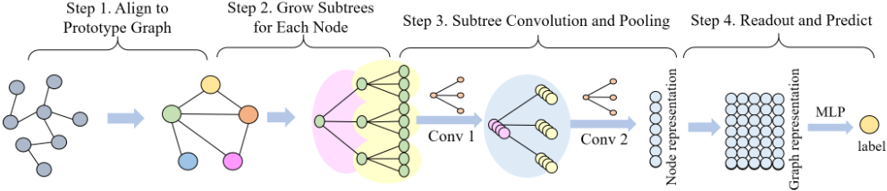
Figure 1 illustrates the process framework of the proposed HA-SCN method. Step 1: Align to Prototype Graph, we align the original graphs with a prototype graph, transforming the arbitrary-sized graphs into fixed-sized aligned graphs. This process establishes nodes correspondences, mitigating the information loss and node order dependency issues in the GNNs. Step 2: Grow Subtrees For Each Node, we employ graph grafting and pruning procedures to grow a normalized K-layer m-ary subtree for each node in the aligned graphs. This step is designed to create a local neighborhood structure for each node, which is essential for the subsequent subtree convolution network. Step 3: Subtree Convolution and Pooling, we perform the subtree convolution and pooling operation by sliding the convolution kernel over the normalized subtrees, achieving weight sharing and progressively reducing the size of the subtrees layer by layer. Step 4: Readout and Predict, a more expressive Multilayer Perceptron (MLP) is used to readout the graph representation and make predictions. Below, we introduce these steps in sequence.
3.1 STEP 1: Aligning to Prototype Graph
In this step, we align the original graphs with the prototype graph, resulting in a set of aligned graphs. Inspired by previous works [Bai et al., 2019; Bai et al., 2022a; Bai et al., 2022b; Bai et al., 2023; Cui et al., 2024], we first cluster the nodes in the graph using the k-means algorithm to obtain prototype nodes. Then, we align the nodes of the original graph with the prototype nodes that have the most similar semantic features, producing an alignment matrix. Finally, we use this alignment matrix to assign the original graph, obtaining a fixed-sized grid structure with nodes that have spatial correspondences.
First, we obtain the node representations of the prototype graph to capture the main features of the nodes in the graph dataset, as shown in Figure 2. Let the graph dataset G = {G1,G2, . . . ,GN} consist of N graphs. Assume that there are n nodes in G, and their feature vectors are represented as R = {R1, R2, . . . , Rn}. We apply the k-means [Witten et al., 2011] algorithm to determine M centroids by minimizing the objective function
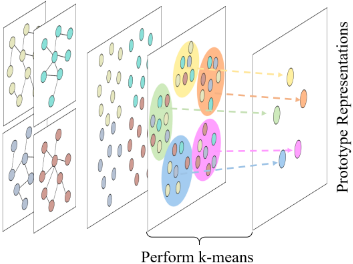
where Ω = {c1, c2, . . . , cM} represents M clusters, and µj is the mean of the node representations belonging to the j-th cluster cj . The set PR = {µ1, µ2, . . . , µM} represents the M prototype node representations of the prototype graph. Next, we compute the distance between the node features of each graph Gp and the prototype node representations. Specifically, each sample graph Gp (where p ∈ {1, . . . ,N}) is represented as Gp(Xp, Ap), with np as the number of nodes, fp as the feature dimension, Xp ∈ Rnp×fp as the node feature matrix, and Ap ∈ {0, 1}np×np as the adjacency matrix. We calculate the distance matrix Dp as
The matrix Dp is a np × M matrix, where each element Dp(i, j) represents the distance between the i-th node representation Rp;i of graph Gp and the prototype node µj ∈ PR. If Dp(i, j) is the smallest in row i, it indicates that node i is closest to the j-th cluster center, and thus, we align the node i with the prototype node j. Based on this, we can construct the corresponding alignment matrix Cp ∈ {0, 1}np×M , i.e.,
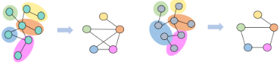
With the corresponding alignment matrix, we align the sample graph Gp(Xp,Ap) with the prototype graph, as two examples are shown in Figure 3. In this step, we adopt an allocation strategy similar to that of the DiffPool [Ying et al., 2018]. The aligned graph ¯Gp( ¯Xp, ¯ Ap) is then defined as
where ¯Xp ∈ RM×fp is the node feature of the aligned graph, ¯ Ap ∈ {0, 1}M×M is the adjacency matrix, ˜ Ap is the adjacency matrix with added self-loops (i.e., ˜ Ap = A + I).
To construct reliable grid structures for graphs, we utilize the depth-based (DB) representations as the node representations, which are defined by calculating the entropies of a series of K-layer expansion subgraphs rooted at a node [Bai and Hancock, 2014]. It is shown that such a DB representation encapsulates rich entropy content flow from each local node to the global graph structure.
3.2 STEP 2: Growing Subtrees for Each Node
In this step, we construct a normalized K-layer m-ary tree for each node. It comprises two steps: (1) construct a m-ary tree for each node by the graph grafting and graph pruning algorithm; (2) The leaf nodes of the i-level m-ary tree are further replaced by their own neighborhood m-ary trees, hence a Klevel m-ary tree is recursively constructed. Below we will introduce these steps.
Constructing the m-ary Tree
To facilitate the use of a fixed-size filter for subtree convolution, we standardize the number of leaf nodes for each node. Given the variability in the number of neighbors for each node, we employ the graph grafting and graph pruning algorithm to construct the m-ary tree.
Graph Grafting. For the node with less than m 1-hop neighbors, we use the graph grafting algorithm to select nodes from its i-hop neighborhood (i ≥ 2) to supplement the m-ary tree. As illustrated in Figure 4, let m = 3, with the starred node as the root. The node requires three leaf nodes, but it has only two 1-hop neighbors. Consequently, nodes are selected from the 2-hop neighborhood. If the 2-hop neighbors are insufficient, nodes are further chosen from the 3-hop neighborhood, continuing this process until the condition is satisfied. If more than m nodes are available, nodes with higher PageRank values are prioritized. Finally, the leaf nodes of the m-ary tree are ranked based on their PageRank.
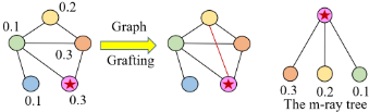
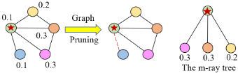
Graph Pruning. For the node with more than m 1-hop neighbors, graph pruning is applied to select the top m nodes with the highest PageRank values. As shown in Figure 5, the starred node has four 1-hop neighbors. The blue node with the lower PageRank is pruned, leaving the remaining three neighbors to form the m-ary tree.
Mapping Graphs to Trees
Through graph grafting and pruning, the subgraph of each node is normalized into an m-ary tree (i.e., the receptive field size of each node is m+ 1). Then we grow the depth of the tree, by recursively replacing their leaf nodes by their own neighborhood m-ary trees, resulting in a K-level m-ary tree for each node. Algorithm 1 details the Mapping Graph to Tree process.
Algorithm 1 Mapping Graph to Tree
Input: Graph, receptive field size m + 1, PageRank algorithm, graph grafting, graph pruning, depth K Output: K-level m-ary tree for each node
- 1: Initialize graph structures.
- 2: Compute PageRank values for each node.
- 3: Construct an m-ary tree for each node using graph grafting and pruning algorithms.
- 4: for i = 2 → i ≤K do
- 5: Replace the leaf nodes of the i-level m-ary tree with their own neighborhood m-ary trees.
- 6: end for
- 7: return K-level m-ary tree for each node.
3.3 STEP 3: The Subtree Convolution and Pooling
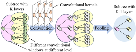
In this subsection, we perform hierarchical subtree convolution and pooling operations on the normalized K-layer m-ary trees, as shown in Figure 6. Specifically, the subtree convolution operation uses a fixed-sized convolution kernel and slides over the subtrees constructed in Step 2 to extract local features. This operation helps capture the structural information within the local neighborhood of each node and enhances the expressive capability of the model through weight sharing. The subtree pooling operation aggregates the features of each subtree, retaining the most important feature information. This operation helps in reducing computational complexity, and hierarchically reducing the size of the subtrees, thereby improving the graph representation capability. Below, we will introduce these two steps in detail.
The Subtree Convolution
We design a convolution operation on the K-layer m-ary trees, where a fixed-sized convolution kernel is used to perform sliding convolution and extract structural features as the output of the convolutional layer. This design is similar to the convolution layers in CNNs, achieving weight sharing and fixed-sized convolution kernels.
As shown in Figure 6, the orange subtree represents subtree convolution kernels containing m + 1 nodes, and each ellipse represents a convolutional window. The convolution operation involves sliding this convolution kernel over each of these ellipses to perform the convolution. Specifically, we use W l ∈ R(m+1)×f l-1×f l to denote the weight matrix of the subtree convolution kernel at layer l, and Xl-1 ∈ R(m+1)×f l-1 to represent the features of the nodes in the convolution receptive field. Here, the number of input feature channels for each node is f l-1 , and the number of output feature channels after applying the subtree convolution is f l . The convolution operation can be defined as
where i corresponds to the input feature dimension, i ∈ {1, . . . , f l-1 }, and ⊙ denotes the element-wise multiplication. bl ∈ R(m+1)×f l is the bias, and f(·) represents an activation function. Y l ∈ R(m+1)×f l is the output of the subtree convolution. This convolution operation means performing a weighted summation for each input feature.
The Subtree Pooling
We perform subtree pooling operations within each subtree receptive field (i.e., the ellipse), pooling the nodes within each field into a single node, thereby reducing the number of nodes and parameters. Traditional graph pooling methods, such as DiffPool [Ying et al., 2018], typically use a GCN layer to learn the clustering information and perform pooling over each cluster. In contrast, our pooling operation directly acts on the output of the previous layer without any preprocessing steps. This allows more efficient processing of the graph structure. The pooling operation is defined as
whereW l ∈ R1×f l and bl ∈ R1×f l are the weight vector and bias of the pooling layer. The function pool(·) is typically defined as either max pooling or average pooling, as commonly used in CNNs.
3.4 STEP 4: Readout and Prediction
After the hierarchical subtree convolution and pooling operations, each subtree is ultimately reduced to a root node. These root nodes are then concatenated to represent the entire graph. We pass this graph feature through an MLP layer to predict the labels of graphs. Since the nodes in the graph have been aligned with the prototype graph in Step 1, we are able to leverage the MLP for prediction, which provides more expressive power compared to the permutation-invariant readout function typically used in the GNNs. To train the model, we use the cross-entropy loss function, which is commonly employed for classification tasks.
3.5 Advantages of the HA-SCNModel
The HA-SCN model offers several key advantages that enhance its performance and efficiency.
First, by iteratively updating cluster centers using k-means, the HA-SCN identifies the most representative nodes in the graph, aligning the nodes of the original graph with the prototype graph nodes that share similar semantics. This alignment process ensures spatial correspondence among the nodes, utilizing information from all nodes in contrast to methods like the SortPool in the DGCNN, which only retains the highestranking nodes. Moreover, the alignment enables the use of an MLP as the readout function, effectively reducing information loss. The process also leads to a reduction in the number of nodes, making the graph more uniform and reducing computational complexity in subsequent steps.
Second, through the growth of subtrees, the HA-SCN constructs normalized K-layer m-ary trees. This technique helps achieve parameter sharing and sliding convolution, while also limiting the size of the receptive field, thus mitigating the over-squashing problem. By performing convolution within a fixed-sized subtree, the model ensures better control over the feature aggregation process.
Third, the HA-SCN employs hierarchical subtree convolution and pooling operations, where each subtree is progressively abstracted layer by layer. Unlike the traditional GNNs, where the receptive field grows exponentially with the number of layers, the HA-SCN maintains a fixed receptive field size as the network deepens. This fixed-size convolution kernel applied within a fixed-sized receptive field further alleviates the over-squashing issue, ensuring that important features are preserved as the network depth increases.
4 Experiments
4.1 Experimental Setups
We evaluate the proposed HA-SCN model on seven benchmark graph classification datasets of two categories: bioinformatics (Bio) and social networks (SN). Detailed descriptions are shown in Table 1. We set the number of nodes in the prototype graph according to the scale of the input graphs. Specifically, we set it to 16 for the MUTAG dataset, 64 for the D&D and REDB datasets, and 32 for the remaining datasets. For each aligned graph, we choose K = 2 and m = 3, constructing a 3-layer binary tree for each node. Our HA-SCN model consists of five layers: one input layer, two subtree convolution pooling layers for extracting node feature information, one MLP layer for integrating graph-level information, and one output layer. In the convolution pooling layers, we set the number of filters to 32. We use the Adam optimization algorithm [Kingma and Ba, 2014] for gradient descent. All weights are randomly initialized from a normal distribution with mean zero and variance 0.01, and we adopt ReLU as the activation function and apply average pooling for readout. To evaluate the classification performance, we perform 10-fold cross-validation, using nine folds for training and one fold for testing. The experiment is repeated 10 times, and we report the average classification accuracies along with the standard errors. Code is available on GitHub. 1
| Dataset | MUTAG | PTC MR | PROTEINS | D&D | IMDB-B | IMDB-M | REDB |
|---|---|---|---|---|---|---|---|
| Max Nodes | 28 | 64 | 620 | 5748 | 136 | 89 | 3782 |
| Avg Nodes | 17.9 | 25.5 | 39.1 | 284.3 | 19.8 | 13 | 429.6 |
| Graphs | 188 | 344 | 1113 | 1178 | 1000 | 1500 | 2000 |
| Classes | 2 | 2 | 2 | 2 | 2 | 3 | 2 |
| Domain | Bio | Bio | Bio | Bio | SN | SN | SN |
We compare the HA-SCN with seven graph kernel methods, eleven advanced GNNs, and four GNNs to address the over-squashing issue. Specifically, the graph kernel methods include: 1) the RWGK [Gartner et al., 2003], 2) GK [Shervashidze et al., 2009], 3) WLSK [Shervashidze et al., 2011], 4) JTQK [Bai et al., 2014], where q = 2, 5) ASK [Bai et al., 2015], 6) EDBMK [Xu et al., 2021], and 7) QBMK [Bai et al., 2024]. The advanced GNNs include: five baseline models-1) the DGCNN [Zhang et al., 2019], 2) DiffPool [Ying et al., 2018], 3) ECC [Simonovsky and Komodakis, 2017], 4) GIN [Xu et al., 2019], and 5) GraphSAGE [Hamilton et al., 2017]-as well as six additional advanced models: 1) the DGK [Yanardag and Vishwanathan, 2015], 2) p-RWNN [Nikolentzos and Vazirgiannis, 2020], with p = 1, 2, 3, and 3) GKNN WL & GKNN GL [Cosmo et al., 2024]. The GNNs addressing the over-squashing issue include: 1) the FA [Alon and Yahav, 2021], 2) SDRF [Topping et al., 2022], 3) FoSR [Karhadkar et al., 2023], and 4) GTR [Black et al., 2023].
4.2 Experimental Results and Discussion
The classification accuracy and standard error of the experiments are shown in Table 2, Table 3, and Table 4. Since the alternative kernels are evaluated with the same setup, we directly use the accuracies from the corresponding literature. For the baseline GNN models, we adapt the results from the fair comparison [Errica et al., 2020]. For other GNNs, we report the best results from their original papers. The Rank column represents the mean ranking of each method.
1 https://github.com/Xiaoqin0421/HA-SCN
Experimental results show that the proposed HA-SCN model outperforms the compared graph kernels, GNNs, and models designed to address the over-squashing. The effectiveness of the proposed HA-SCN is threefold.
First, the HA-SCN aligns nodes to a prototype graph, preserving structural correspondence and enhancing node feature expressiveness. This overcomes the limitations of the GNNs and the graph kernels which ignore the nodematching information, significantly boosting classification performance. Second, although the ASK, the EDBMK, and the QBMK kernels consider node-matching information, they perform pairwise graph alignment. In contrast, our model aligns sample graphs with a prototype graph, improving the alignment efficiency. Additionally, we utilize a deep learning model for learning, which is more effective for learning compared to shallow C-SVM models for feature extraction. Third, the HA-SCN employs a subtree convolution and pooling mechanism that provides each node with a fixed-sized receptive field, preventing excessive information aggregation and mitigating the over-squashing.
4.3 Hyperparameter Analysis
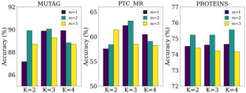
We perform hyperparameter analysis to study the size of the subtrees. Specifically, we vary the number of layers K and the number of leaf nodes m, evaluating their impact on performance. Using the MUTAG, PTC MR, and PROTEINS datasets as examples, we test on K = 2, 3, 4 and m = 1, 2, 3, with the results presented in Figure 7.
Based on the experimental results, we find that the HASCN model performs best with a 3-layer binary tree structure. Specifically, the number of leaf nodes has a significant impact on model performance. When the number of leaf nodes decreases, the receptive field of each node becomes smaller, making it difficult to capture sufficient local structural information, which affects feature extraction and reduces classification accuracy. On the other hand, increasing the number of leaf nodes may dilute effective node features and introduce noise, and the additional weight parameters can lead to overfitting, decreasing the generalization ability of the model.
| MUTAG | PTC MR | PROTEINS | D&D | IMDB B | IMDB M | REDB | Rank | |
|---|---|---|---|---|---|---|---|---|
| HA-SCN | 90.05±1.14(1) | 63.18±1.47(1) | 76.28±0.27(1) | 79.29±0.39(1) | 73.20±0.37(1) | 49.87±0.60(1) | 88.67±0.25(6) | 1.71 |
| DGCNN | - | - | 72.9±3.5(10) | 76.6±4.3(6) | 69.2±3.0(8) | 45.6±3.4(9) | 87.8±2.5(7) | 8.00 |
| DiffPool | - | - | 73.7±3.5(7) | 75.0±3.5(8) | 68.4±3.3(10) | 45.6±3.4(9) | 89.1±1.6(5) | 7.80 |
| ECC | - | - | 72.3±3.4(11) | 72.6±4.1(10) | 67.7±2.8(11) | 43.5±3.1(11) | - | 10.75 |
| GIN | - | - | 73.3±4.0(8) | 75.3±2.9(7) | 71.2±3.9(2) | 48.5±3.3(3) | 89.9±1.9(3) | 4.60 |
| GraphSAGE | - | - | 73.0±4.5(9) | 72.9±2.0(9) | 68.8±4.5(9) | 47.6±3.5(7) | 84.3±1.9(8) | 8.40 |
| DGK | 82.66±1.45(7) | 57.32±1.13(4) | 71.68±0.50(12) | 78.50±0.22(2) | 66.96±0.56(12) | 44.55±0.52(10) | 77.34±0.18(9) | 8.00 |
| 1-RWNN | 89.2±4.3(2) | - | 75.7±3.3(2) | 77.6±4.7(3) | 70.8±4.8(3) | 47.8±3.8(6) | 90.4±1.9(1) | 2.83 |
| 2-RWNN | 88.1±4.8(4) | - | 74.1±3.3(6) | 76.9±4.6(5) | 70.6±4.4(5) | 48.8±2.9(2) | 90.3±1.8(2) | 4.00 |
| 3-RWNN | 88.6±4.1(3) | - | 74.3±3.3(5) | 77.4±4.9(4) | 70.7±3.9(4) | 47.8±3.5(5) | 89.7±1.2(4) | 4.12 |
| GKNNWL | 85.73±2.70(5) | 59.29±2.54(3) | 74.94±1.10(4) | - | 69.7±2.20(7) | 47.87±1.78(4) | - | 4.60 |
| GKNNGL | 85.24±2.28(6) | 60.13±1.94(2) | 75.36±1.12(3) | - | 69.90±1.44(6) | 45.67±1.22(8) | - | 5.00 |
| MUTAG | PTC MR | PROTEINS | D&D | IMDB B | IMDB M | REDB | Rank | |
|---|---|---|---|---|---|---|---|---|
| HA-SCN | 90.05±1.14(1) | 63.18±1.47(1) | 76.28±0.27(1) | 79.29±0.39(3) | 73.20±0.37(1) | 49.87±0.60(3) | 88.67±0.25(1) | 1.57 |
| RWGK | 80.77±0.72(8) | 55.91±0.37(6) | 74.20±0.40(2) | 71.70±0.47(7) | 67.94±0.77(5) | 46.72±0.30(5) | 72.73±0.39(5) | 5.42 |
| GK | 81.66±0.11(7) | - | 71.67±0.55(5) | 78.65±0.27(4) | 73.19±0.23(2) | 45.42±0.87(6) | 77.34±0.18(3) | 4.50 |
| WLSK | 82.88±0.57(6) | 56.05±0.51(5) | 73.52±0.43(3) | 79.78±0.36(1) | 71.88±0.77(4) | 49.50±0.49(4) | 76.56±0.30(4) | 3.85 |
| JTQK | 85.50±0.55(5) | 57.39±0.46(3) | 72.86±0.41(4) | 79.49±0.32(2) | 72.45±0.81(3) | 50.33±0.49(1) | 77.60±0.35(2) | 2.85 |
| ASK | 87.50±0.65(3) | - | - | 70.38±0.72(8) | - | 50.12±0.51(2) | - | 4.33 |
| EDBMK | 86.35(4) | 56.75(4) | - | 78.19(5) | - | - | - | 4.33 |
| QBMK | 88.55±0.43(2) | 59.38±0.36(2) | - | 77.60±0.47(6) | - | - | - | 3.33 |
| MUTAG | PROTEINS | IMDB B | REDB | Rank | |
|---|---|---|---|---|---|
| HA-SCN | 90.05±1.14(1) | 76.28±0.27(1) | 73.20±0.37(1) | 88.67±0.25(4) | 1.75 |
| FA | 83.45±1.74(4) | 72.30±0.67(4) | 71.48±0.88(4) | 90.22±0.48(3) | 3.75 |
| SDRF | 82.70±1.78(5) | 70.92±0.79(5) | 70.21±0.81(5) | 86.83±0.52(5) | 5.00 |
| FoSR | 86.15±1.49(2) | 75.25±0.86(3) | 71.96±0.69(2) | 90.94±0.47(1) | 2.00 |
| GTR | 86.10±1.76(3) | 75.78±0.76(2) | 71.49±0.93(3) | 90.41±0.41(2) | 2.50 |
Regarding tree depth, if the number of layers is too small, the model fails to capture deep graph structural features, leading to insufficient representation of hierarchical features and negatively impacting classification performance. Conversely, too many layers may cause excessive information compression, leading to the loss of important details. Therefore, the 3-layer binary tree structure provides an appropriate receptive field, with subtree of each node containing 7 nodes, effectively covering sufficient local structural information and allowing the model to perform optimally in classification tasks.
4.4 Visualization
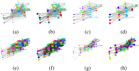
In Figure 8, we visualize the effect of graph alignment of the proposed HA-SCN model. Figures (a)-(d) and (e)-(h) display examples from the PROTEINS and D&D datasets, respectively, where different colors represent different clusters. Figures (a), (c), (e), and (g) show the original graph structure (gray edges), while the corresponding graphs on the right overlay the aligned structure, with larger nodes and black edges indicating the nodes and edges in the aligned graph. From these figures, it can be seen that nodes with similar representations are effectively assigned to the same cluster. This alignment not only helps aggregate similar nodes, but also establishes clearer correspondences between the nodes.
5 Conclusion
In this paper, we have proposed a novel HA-SCN model for graph classification, overcoming the limitations of the traditional GNNs. Our method introduces a novel approach that transforms graphs into fixed-sized aligned grid structures, establishing spatial correspondence between nodes. By defining a new subtree convolution and pooling operation, we hierarchically abstract node information, allowing the model to capture deeper graph features. This approach effectively mitigates the over-squashing problem commonly encountered in GNNs, enabling more stable and efficient learning. Additionally, the HA-SCN implements effective weight sharing and uses fixed-sized convolution filters, further enhancing its performance. Experiments on benchmark graph datasets demonstrate the superior classification performance of the HA-SCN. In future work, we will explore the use of other aligned substructures, such as paths and cycles, and design more effective and specialized convolutional strategies.
Acknowledgments
This work is supported by the National Natural Science Foundation of China under Grants T2122020, 61602535, and 62172370. This work is also supported in part by the Jinhua Science and Technology Plan (No. 2023-3-003a), the Humanity and Social Science Foundation of Ministry of Education (24YJAZH022), and the Program for Innovation Research in the Central University of Finance and Economics.
@inproceedings{ijcai2025p361,
  title     = {HA-SCN: Learning Hierarchical Aligned Subtree Convolutional Networks for Graph Classification},
  author    = {Qin, Xinya and Bai, Lu and Cui, Lixin and Li, Ming and Du, Hangyuan and Wang, Yue and Hancock, Edwin},
  booktitle = {Proceedings of the Thirty-Fourth International Joint Conference on
               Artificial Intelligence, {IJCAI-25}},
  publisher = {International Joint Conferences on Artificial Intelligence Organization},
  editor    = {James Kwok},
  pages     = {3245--3253},
  year      = {2025},
  month     = {8},
  note      = {Main Track},
  doi       = {10.24963/ijcai.2025/361},
  url       = {https://doi.org/10.24963/ijcai.2025/361},
}
TY - CPAPER TI - HA-SCN: Learning Hierarchical Aligned Subtree Convolutional Networks for Graph Classification AU - Qin, Xinya AU - Bai, Lu AU - Cui, Lixin AU - Li, Ming AU - Du, Hangyuan AU - Wang, Yue AU - Hancock, Edwin T2 - Proceedings of the Thirty-Fourth International Joint Conference on Artificial Intelligence, IJCAI-25 PB - International Joint Conferences on Artificial Intelligence Organization PY - 2025 SP - 3245 EP - 3253 DO - 10.24963/ijcai.2025/361 UR - https://doi.org/10.24963/ijcai.2025/361 ER -Copied
Machine-readable versions of this paper, for tools and AI agents:





