
DualCast: A Model to Disentangle Aperiodic Events from Traffic Series
Proceedings of the Thirty-Fourth International Joint Conference on Artificial Intelligence. Main Track. Pages 3290-3298.
https://doi.org/10.24963/ijcai.2025/366
Keywords
- Data Mining: DM: Frequent pattern mining
- Data Mining: DM: Mining spatial and/or temporal data
Abstract
Traffic forecasting is crucial for transportation systems optimisation. Current models minimise the mean forecasting errors, often favouring periodic events prevalent in the training data, while overlooking critical aperiodic ones like traffic incidents. To address this, we propose DualCast, a dual-branch framework that disentangles traffic signals into intrinsic spatial-temporal patterns and external environmental contexts, including aperiodic events. DualCast also employs a cross-time attention mechanism to capture high-order spatial-temporal relationships from both periodic and aperiodic patterns. DualCast is versatile. We integrate it with recent traffic forecasting models, consistently reducing their forecasting errors by up to 9.6% on multiple real datasets.
- [Arevalo et al., 2017] John Arevalo, Thamar Solorio, Manuel Montes-y Gómez, and Fabio A González. Gated Multimodal Units for Information Fusion. arXiv preprint arXiv:1702.01992, 2017.
- [Box et al., 2015] George E. P. Box, Gwilym M. Jenkins, Gregory C. Reinsel, and Greta M. Ljung. Time Series Analysis: Forecasting and Control. John Wiley & Sons, 2015.
- [Chang et al., 2024] Ching Chang, Chiao-Tung Chan, Wei- Yao Wang, Wen-Chih Peng, and Tien-Fu Chen. Time- DRL: Disentangled Representation Learning for Multi- variate Time-Series. In ICDE, 2024.
- [Chen et al., 2021] Xinqiang Chen, Huixing Chen, Yong- sheng Yang, Huafeng Wu, Wenhui Zhang, Jiansen Zhao, and Yong Xiong. Traffic Flow Prediction by an Ensem- ble Framework with Data Denoising and Deep Learning Model. Physica A: Statistical Mechanics and Its Applica- tions, 2021.
- [Davies and Bouldin, 1979] David L Davies and Donald W Bouldin. A Cluster Separation Measure. IEEE Transac- tions on Pattern Analysis and Machine Intelligence, 1979.
- [Deng et al., 2021] Jinliang Deng, Xiusi Chen, Renhe Jiang, Xuan Song, and Ivor W Tsang. ST-Norm: Spatial and Temporal Normalization for Multi-variate Time Series Forecasting. In KDD, 2021.
- [Dey et al., 2023] Subhrasankha Dey, Stephan Winter, Mar- tin Tomko, and Niloy Ganguly. Traffic Count Estimation at Basis Links without Path Flow and Historic Data. IEEE Transactions on Intelligent Transportation Systems, 2023.
- [Fang et al., 2021] Zheng Fang, Qingqing Long, Guojie Song, and Kunqing Xie. Spatial-Temporal Graph ODE Networks for Traffic Flow Forecasting. In KDD, 2021.
- [Fang et al., 2023] Yuchen Fang, Yanjun Qin, Haiyong Luo, Fang Zhao, Bingbing Xu, Liang Zeng, and Chenxing Wang. When Spatio-Temporal Meet Wavelets: Disentan- gled Traffic Forecasting via Efficient Spectral Graph At- tention Networks. In ICDE, 2023.
- [Guo et al., 2019] Shengnan Guo, Youfang Lin, Ning Feng, Chao Song, and Huaiyu Wan. Attention Based Spatial- Temporal Graph Convolutional Networks for Traffic Flow Forecasting. In AAAI, 2019.
- [Hochreiter and Schmidhuber, 1997] Sepp Hochreiter and Jürgen Schmidhuber. Long Short-Term Memory. Neural Computation, 1997.
- [Huang et al., 2023] Siyuan Huang, Yunchong Song, Jiayue Zhou, and Zhouhan Lin. Tailoring Self-Attention for Graph via Rooted Subtrees. In NeurIPS, 2023.
- [Jiang et al., 2023a] Jiawei Jiang, Chengkai Han, Wayne Xin Zhao, and Jingyuan Wang. PDFormer: Propagation Delay-Aware Dynamic Long-Range Transformer for Traf- fic Flow Prediction. In AAAI, 2023.
- [Jiang et al., 2023b] Renhe Jiang, Zhaonan Wang, Jiawei Yong, Puneet Jeph, Quanjun Chen, Yasumasa Kobayashi, Xuan Song, Shintaro Fukushima, and Toyotaro Suzumura. Spatio-Temporal Meta-Graph Learning for Traffic Fore- casting. In AAAI, 2023.
- [Jin et al., 2022] Yilun Jin, Kai Chen, and Qiang Yang. Se- lective Cross-City Transfer Learning for Traffic Prediction via Source City Region Re-Weighting. In KDD, 2022.
- [Jin et al., 2023] Yilun Jin, Kai Chen, and Qiang Yang. Transferable Graph Structure Learning for Graph-based Traffic Forecasting across Cities. In KDD, 2023.
- [Karacasu et al., 2011] Murat Karacasu, Arzu Er, Safak Bil- gic, and Hasan B Barut. Variations in Traffic Accidents on Seasonal, Monthly, Daily and Hourly Basis: Eskisehir Case. Procedia-Social and Behavioral Sciences, 2011.
- [Kong et al., 2024] Weiyang Kong, Ziyu Guo, and Yubao Liu. Spatio-Temporal Pivotal Graph Neural Networks for Traffic Flow Forecasting. In AAAI, 2024.
- [Kumar and Vanajakshi, 2015] S Vasantha Kumar and Lelitha Vanajakshi. Short-Term Traffic Flow Prediction Using Seasonal ARIMA Model with Limited Input Data. European Transport Research Review, 2015.
- [Li and Zhu, 2021] Mengzhang Li and Zhanxing Zhu. Spatial-Temporal Fusion Graph Neural Networks for Traf- fic Flow Forecasting. In AAAI, 2021.
- [Li et al., 2018] Yaguang Li, Rose Yu, Cyrus Shahabi, and Yan Liu. Diffusion Convolutional Recurrent Neural Net- work: Data-Driven Traffic Forecasting. In ICLR, 2018.
- [Li et al., 2024] Shuhao Li, Yue Cui, Libin Li, Weidong Yang, Fan Zhang, and Xiaofang Zhou. ST-ABC: Spatio- Temporal Attention-Based Convolutional Network for Multi-Scale Lane-Level Traffic Prediction. In ICDE, 2024.
- [Liu et al., 2022] Xu Liu, Yuxuan Liang, Chao Huang, Yu Zheng, Bryan Hooi, and Roger Zimmermann. When do Contrastive Learning Signals Help Spatio-temporal Graph Forecasting? In SIGSPATIAL, 2022.
- [Liu et al., 2023] Hangchen Liu, Zheng Dong, Renhe Jiang, Jiewen Deng, Jinliang Deng, Quanjun Chen, and Xuan Song. Spatio-temporal Adaptive Embedding Makes Vanilla Transformer SOTA For Traffic Forecasting. In CIKM, 2023.
- [Ma et al., 2024] Minbo Ma, Jilin Hu, Christian S Jensen, Fei Teng, Peng Han, Zhiqiang Xu, and Tianrui Li. Learn- ing Time-aware Graph Structures for Spatially Correlated Time Series Forecasting. In ICDE, 2024. [
- [PeMS, 2001] PeMS. https://pems.dot.ca.gov, 2001. Link
- [Qi et al., 2022] Jianzhong Qi, Zhuowei Zhao, Egemen Tanin, Tingru Cui, Neema Nassir, and Majid Sarvi. A Graph and Attentive Multi-Path Convolutional Network for Traffic Prediction. IEEE Transactions on Knowledge and Data Engineering, 2022.
- [Qin et al., 2024] Jianyang Qin, Yan Jia, Yongxin Tong, Heyan Chai, Ye Ding, Xuan Wang, Binxing Fang, and Qing Liao. MUSE-Net: Disentangling Multi-Periodicity for Traffic Flow Forecasting. In ICDE, 2024.
- [Ruikar, 2013] Manisha Ruikar. National Statistics of Road Traffic Accidents in India. Journal of Orthopaedics, Trau- matology and Rehabilitation, 2013.
- [Song et al., 2020] Chao Song, Youfang Lin, Shengnan Guo, and Huaiyu Wan. Spatial-Temporal Synchronous Graph Convolutional Networks: A New Framework for Spatial- Temporal Network Data Forecasting. In AAAI, 2020.
- [Su et al., 2024a] Xinyu Su, Feng Liu, Yanchuan Chang, Egemen Tanin, Majid Sarvi, and Jianzhong Qi. DualCast: Disentangling Aperiodic Events from Traffic Series with a Dual-Branch Model. arXiv preprint arXiv:2411.18286, 2024.
- [Su et al., 2024b] Xinyu Su, Jianzhong Qi, Egemen Tanin, Yanchuan Chang, and Majid Sarvi. Spatial-Temporal Forecasting for Regions without Observations. In EDBT, 2024.
- [Sun et al., 2024] Ke Sun, Pei Liu, Pengfei Li, and Zhifang Liao. ModWaveMLP: MLP-Based Mode Decomposition and Wavelet Denoising Model to Defeat Complex Struc- tures in Traffic Forecasting. In AAAI, 2024.
- [Tang et al., 2024] Yujin Tang, Lu Qi, Fei Xie, Xiangtai Li, Chao Ma, and Ming-Hsuan Yang. PredFormer: Trans- formers Are Effective Spatial-Temporal Predictive Learn- ers. arXiv preprint arXiv:2410.04733, 2024.
- [Tian and Pan, 2015] Yongxue Tian and Li Pan. Predicting Short-term Traffic Flow by Long Short-term Memory Re- current Neural Network. In IEEE International Confer- ence on Smart City/SocialCom/SustainCom, 2015.
- [Victoria Road Crash Data, 2023] Victoria Road Crash Data. https://discover.data.vic.gov.au/dataset/ victoria-road-crash-data, 2023. Link
- [Wang et al., 2020] Xiaoyang Wang, Yao Ma, Yiqi Wang, Wei Jin, Xin Wang, Jiliang Tang, Caiyan Jia, and Jian Yu. Traffic Flow Prediction via Spatial Temporal Graph Neural Network. In WWW, 2020.
- [Wang et al., 2021] Jingyuan Wang, Jiawei Jiang, Wenjun Jiang, Chao Li, and Wayne Xin Zhao. LibCity: An Open Library for Traffic Prediction. In SIGSPATIAL, 2021.
- [Wang et al., 2022] Zhaonan Wang, Renhe Jiang, Hao Xue, Flora D Salim, Xuan Song, and Ryosuke Shibasaki. Event- aware Multimodal Mobility Nowcasting. In AAAI, 2022.
- [Wu et al., 2019] Zonghan Wu, Shirui Pan, Guodong Long, Jing Jiang, and Chengqi Zhang. Graph WaveNet for Deep Spatial-Temporal Graph Modeling. In IJCAI, 2019. IJCAI
- [Wu et al., 2020] Zonghan Wu, Shirui Pan, Guodong Long, Jing Jiang, Xiaojun Chang, and Chengqi Zhang. Connect- ing the Dots: Multivariate Time Series Forecasting with Graph Neural Networks. In KDD, 2020.
- [Xia et al., 2023] Yutong Xia, Yuxuan Liang, Haomin Wen, Xu Liu, Kun Wang, Zhengyang Zhou, and Roger Zimmer- mann. Deciphering Spatio-Temporal Graph Forecasting: A Causal Lens and Treatment. NeurIPS, 2023.
- [Xu et al., 2020] Mingxing Xu, Wenrui Dai, Chunmiao Liu, Xing Gao, Weiyao Lin, Guo-Jun Qi, and Hongkai Xiong. Spatial-Temporal Transformer Networks for Traffic Flow Forecasting. arXiv preprint arXiv:2001.02908, 2020.
- [Yi et al., 2024] Kun Yi, Qi Zhang, Wei Fan, Hui He, Liang Hu, Pengyang Wang, Ning An, Longbing Cao, and Zhen- dong Niu. FourierGNN: Rethinking Multivariate Time Series Forecasting from a Pure Graph Perspective. In NeurIPS, 2024.
- [Yu et al., 2018] Bing Yu, Haoteng Yin, and Zhanxing Zhu. Spatio-Temporal Graph Convolutional Networks: A Deep Learning Framework for Traffic Forecasting. In IJCAI, 2018. IJCAI
- [Zhao et al., 2017] Zheng Zhao, Weihai Chen, Xingming Wu, Peter CY Chen, and Jingmeng Liu. LSTM Network: A Deep Learning Approach for Short-Term Traffic Fore- cast. IET Intelligent Transport Systems, 2017.
- [Zhao et al., 2023] Yusheng Zhao, Xiao Luo, Wei Ju, Chong Chen, Xian-Sheng Hua, and Ming Zhang. Dynamic Hy- pergraph Structure Learning for Traffic Flow Forecasting. In ICDE, 2023.
- [Zheng et al., 2020] Chuanpan Zheng, Xiaoliang Fan, Cheng Wang, and Jianzhong Qi. GMAN: A Graph Multi-Attention Network for Traffic Prediction. In AAAI, 2020.
- [Zheng et al., 2023] Chuanpan Zheng, Xiaoliang Fan, Cheng Wang, Jianzhong Qi, Chaochao Chen, and Long- biao Chen. INCREASE: Inductive Graph Representation Learning for Spatio-Temporal Kriging. In WWW, 2023.
- [Zhou et al., 2023] Zhengyang Zhou, Qihe Huang, Kuo Yang, Kun Wang, Xu Wang, Yudong Zhang, Yuxuan Liang, and Yang Wang. Maintaining the Status Quo: Cap- turing Invariant Relations for OOD Spatiotemporal Learn- ing. In KDD, 2023.
References were extracted automatically from the PDF and may contain errors.
Full text extracted automatically from the PDF; figures, tables and equations may differ. The PDF is the version of record.
1 Introduction
Traffic forecasting is essential for intelligent transportation systems (ITS), enabling real-time solutions like route planning and transportation scheduling.
Deep learning-based solutions have dominated the traffic forecasting literature in recent years. They typically adopt graph neural networks (GNNs) for modelling spatial patterns and sequential models for modelling temporal patterns [Song et al., 2020; Wang et al., 2020; Li and Zhu, 2021; Fang et al., 2021; Liu et al., 2022; Qi et al., 2022]. Besides, a series of recent studies adopt the attention mechanism to capture dynamic relationships in traffic patterns [Guo et al., 2019; Liu et al., 2023; Tang et al., 2024].
These solutions are primarily designed to minimise mean forecasting errors, a common evaluation metric [Xu et al., 2020; Zheng et al., 2020; Jiang et al., 2023a]. This optimisation focuses on periodic traffic patterns, which are both easier to forecast and more prevalent in the traffic data, resulting in an easier reduction in mean errors.
These models struggle with rare and random aperiodic events, such as traffic incidents, making them difficult to forecast. However, promptly identifying and adapting to such events is essential for effective real-time traffic forecasting.
∗Corresponding author.
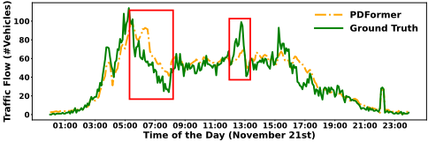
Fig. 1 shows PDFormer [Jiang et al., 2023a] forecasting the traffic flow on a California freeway 60 minutes ahead for one day (detailed in Section 5.2). There are two substantial gaps between the forecasts (the orange dashed line) and ground truth (the green solid line) at around 07:00 and 13:00. These gaps would be overlooked if only mean forecasting error is considered, as the overall patterns are similar.
In this paper, we propose DualCast - a model framework to address the issue above. DualCast is not yet another traffic forecasting model. Instead, we aim to present a generic structure to power current traffic forecasting models with stronger learning capability to handle aperiodic patterns from traffic series. DualCast has a dual-branch design to disentangle a traffic observation into two signals: (1) the intrinsic branch learns intrinsic (periodic) spatial-temporal patterns, and (2) the environment branch learns external environment contexts that contain aperiodic patterns. We implement DualCast with three representative traffic forecasting models, that is, STTN [Xu et al., 2020], GMAN [Zheng et al., 2020] and PDFormer [Jiang et al., 2023a], due to their reported strong learning outcomes.
The success of our dual-branch framework relies on three loss functions: filter loss, environment loss, and DBI loss. These functions guide DualCast to disentangle the two types of signals and later fuse the learning outcomes to generate the forecasting results.
(1) The filter loss computes the reciprocal of KullbackLeibler (KL) divergence between the feature representations learned from two branches, ensuring that each branch captures distinct signals from the input. (2) The environment loss is designed for the environment branch. It computes the reciprocal of KL divergence between a batch of training samples and a randomly permuted sequence of those samples in the same batch. This loss encourages DualCast to learn the diverse environment contexts at different times, as the samples of the training pair used in the KL divergence are drawn from different periods. (3) The DBI loss is designed for the intrinsic branch. It encourages DualCast to learn more separated representations for training samples with different (periodic) traffic patterns while closer representations for samples within the same traffic patterns.
The three models [Xu et al., 2020; Zheng et al., 2020; Jiang et al., 2023a] with which DualCast is implemented all use self-attention. To enhance their self-attention modules to capture spatial-temporal correlations, we identify two issues: (1) Existing self-attention-based models [Xu et al., 2020; Zheng et al., 2020; Jiang et al., 2023a] learn spatial and temporal patterns separately, focusing on nodes at the same time step or the same node across time. They neglect correlations between different nodes across time, while such correlations are important for modelling the impact of aperiodic events like the impact of traffic incidents propagating spatially over time. (2) Existing models take either a local attention [Jiang et al., 2023a] or a global attention [Zheng et al., 2020] setup. They compute attention only among connected nodes (based on the adjacency matrix) or among all nodes. This limits receptive fields or loses hierarchical relationships critical for traffic flow propagation.
To address these issues, we propose: (1) a cross-time attention module using hierarchical message passing based on a conceptual space-time tree, enabling attention across nodes and time steps to better model spatial-temporal traffic propagation without extra storage or computational overhead. (2) an attention fusion module to combine local and global attention, expanding the receptive field and capturing hierarchical node relationships.
Overall, this paper makes the following contributions:
- We propose DualCast - a model framework equipped with two branches and three loss functions to disentangle complex traffic observations into two types of signals for more accurate forecasting. DualCast is versatile in terms of the models to form its two branches - we use self-attentionbased models for their reported strong learning outcomes.
- We propose two enhancements for self-attention-based forecasting models: (i) A cross-time attention module to capture high-order spatial-temporal correlations, and (ii) An attention fusion module to combine global and local attention, enlarging DualCast's receptive field and learning the hierarchical relationships among the nodes.
- We conduct experiments on both freeway and urban traffic datasets, integrating DualCast with three self-attentionbased models GMAN, STTN, and PDFormer. The results show that: (i) DualCast consistently reduces the forecasting errors for these models, with stronger improvements at times with more complex environment contexts and by up to 9.6% in terms of RMSE; (ii) DualCast also outperforms the SOTA model consistently and by up to 2.6%. Our source code is available at https://github.com/suzy0223/DualCast.
2 RelatedWork
Traffic forecasting typically employs sequence models [Box et al., 2015; Hochreiter and Schmidhuber, 1997; Wu et al., 2019] to capture temporal patterns and GNNs for spatial correlations [Tian and Pan, 2015; Kumar and Vanajakshi, 2015; Zhao et al., 2017; Yu et al., 2018; Jin et al., 2022; Zheng et al., 2023; Ma et al., 2024; Su et al., 2024b]. Spatial and temporal layers can be arranged sequentially or in parallel, and fused via methods such as gated fusion [Arevalo et al., 2017]. Some GNN-based models [Zhao et al., 2023] connect graph snapshots over time to reduce the negative impact of the ripple effect, which still overlooks time-varying relationships. Self-attention based traffic forecasting models handle this issue easily [Liu et al., 2023; Li et al., 2024].
Moreover, some studies disentangle traffic series into periodic components [Chen et al., 2021; Deng et al., 2021; Fang et al., 2023; Qin et al., 2024; Sun et al., 2024; Yi et al., 2024], different levels [Chang et al., 2024], or invariant and environment signals [Xia et al., 2023; Zhou et al., 2023]. Others adopt memory augmentation to enhance sensitivity to aperiodic signals [Wang et al., 2022; Jiang et al., 2023b]. Our proposed DualCast employs a dualbranch structure with three loss functions and cross-time attention to flexibly capture diverse, aperiodic patterns and environment contexts without relying on predefined patterns. A full discussion is provided in Appendix A of our online technical report [Su et al., 2024a].
3 Preliminaries
Traffic forecasting. We model a network of traffic sensors as a graph G = (V,E,A), where V denotes a set of N nodes (each representing a sensor) and E denotes a set of edges representing the spatial connectivity between the sensors based on the underlying road network. A ∈ RN×N is an adjacency matrix derived from the graph. If vi, vj ∈ V and (vi, vj) ∈ E, then Ai,j = 1; otherwise, Ai,j = 0.
For each sensor (i.e., a node hereafter, for consistency) vi ∈ V , we use xi,t ∈ RC to represent the traffic observation of vi at time step t, where C is the number of types of observations, e.g., traffic flow and traffic speed. Further, Xt = [x1,t, x2,t . . . , xN,t] ∈ RN×C denotes the observations of all nodes in G at time step t, while ˆXt ∈ RN×C denotes the forecasts of the nodes in G at time step t. We use Xti:tj to denote the consecutive observations from ti to tj.
Problem statement. Given a sensor graph G = (V,E,A), a traffic forecasting model generally adopts an encoderdecoder structure to learn from the traffic observations of the previous T steps and generate forecasts for the following T ′ steps ˆXt+1 : t+T ′ = gω(fθ(Xt-T+1 : t)), where fθ and gω denote the encoder and the decoder, respectively, and θ ∈ Θ and ω ∈ Ω denote the learnable parameters. We aim to find fθ and gω to minimise the errors between the ground-truth observations and the forecasts:
where T denotes the time range of traffic observations of the dataset, and p is commonly set as 1 or 2.
We propose a model optimisation framework named DualCast compatible with recent self-attention-based (STF hereafter) models [Xu et al., 2020; Zheng et al., 2020; Jiang et al., 2023a]. Due to space limit, we detail these models in our technical report [Su et al., 2024a] (Appendix B).
4 The DualCast Framework
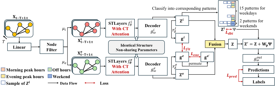
Fig. 2 shows our proposed DualCast with a dual branch structure (Section 4.1), which disentangles traffic observations into two types of underlying signals, namely intrinsic (periodic) signals and environmental (aperiodic) signals for accurate traffic forecasting. We introduce three loss functions: filter loss, environment loss, and DBI loss, to guide the model to generate distinct representations for these signals.
As self-attention-based traffic forecasting models have competitive performance, we use them as baseline models. We design rooted sub-tree cross-time attention (CT attention) module (Section 4.2) which can efficiently capture dynamic and high-order spatial-temporal correlations between sensors on both branches to enhance their performance.
4.1 Dual-branch Structure and Optimisation
Dual-branch structure. The dual-branch structure disentangles the traffic observations into intrinsic and environment signals. The intrinsic branch (IBranch) and environment branch (EBranch) share an identical structure with separate parameters. The intrinsic signals reflect intrinsic (periodic) traffic patterns, while the environment signals reflect external environment (aperiodic) contexts, such as traffic incidents. The two signals together determine the traffic forecasts.
Given a batch of input observations X ∈ RB×T×N×C , we compute disentangling coefficients µi, µe for intrinsic and environment signals as µi, µe = softmax(Linear(X)), where Linear denotes a linear layer with an output size of 2; Both µi and µe have shape RB×T×N . Then, we produce the intrinsic signals Xi = µi ⊙ X and the environment signals Xe = µe ⊙X, where ⊙ is element-wise product, and µi, µe are expanded along the last dimension. These signals are fed into IBranch and EBranch to generate representations Zi and Ze , respectively. The process is detailed for IBranch, with EBranch operating similarly.
In IBranch, Xi is fed into the spatial-temporal encoder f i θ to produce a hidden representation Hi , which is passed to the decoder giω to produce the output representation of the branch, Zi ∈ RB×T×N×D . We concatenate the outputs of both branches to obtain Z = Concat(Zi ,Ze ) and generate the forecasts ˆX fromZ through another linear layer gout ω .
Model training. We train DualCast using three loss functions: (1) filter loss to separate branch feature spaces, (2) environment loss to learn the impact of environment contexts, and (3) DBI loss to learn different periodic patterns.
Filter loss. Denoted as Lflt, is based on KL divergence. It encourages each branch to capture distinct signals. We aggregate the output Zi from IBranch along the time dimension by a linear layer and then along node with mean pooling to produce an overall representation gi ∈ RB×D of each input sample. This process is denoted as riδ , where δ refers to linear layer parameters. Similarly, we obtain ge through re δ from EBranch. We use softmax(·) to map ge and gi into distribution and compute the filter loss as follows:
Environment loss. Denoted as Lenv, guides the EBranch to learn external environment signals (aperiodic events). Our intuition is that the environment context of different samples from different time periods should be random and hence different (otherwise this becomes a periodic signal). To capture such varying environment contexts, the environment loss guides different samples to generate different environment representations. We randomly permute ge along the batch dimension to obtain ge′ = π(ge ). We then obtain B sample pairs (ge i , ge′ i ), i ∈ [1,B]. We use softmax(·) to map ge and ge′ . We aim to separate the representations of the sample pairs to guide DualCast to generate diverse environment representations for different times. Thus:

DBI loss. Denoted as Ldbi and inspired by the Davies-Bouldin index (DBI) [Davies and Bouldin, 1979], guides IBranch to learn representative intrinsic patterns. Traffic observations exhibit different periodic patterns based on time (e.g., workdays vs. weekends, and peak hours vs. off hours). We define 17 time-based patterns (Fig. 3): 15 for workdays (morning peak, off-hour, and evening peak for each weekday), one for Saturdays, and one for Sundays, due to the reduced variation on weekends [Jin et al., 2023; Dey et al., 2023]. Public holidays are treated as Sundays. The output Zi of IBranch contains B samples. We classify each sample based on its start time into one of the 17 patterns. This gives a set of sample representations for each pattern. Let P denote the set of 17 patterns, and p ∈ P refer to one such set. We define a matrix Ψ ∈ R|P|×T×N×D as the prototype for 17 patterns and optimise Ψ during training. The intuition of Ψ is that each of 17 patterns may consist of T distinct sub-patterns for each node, with each sub-pattern represented as a D-dimensional vector. The DBI loss guides DualCast to learn more separated representations for the training samples with different periodic patterns, and closer representations for those with the same periodic patterns. We first compute two metrics S and P that evaluate the compactness of a pattern and the separation among patterns, respectively.
Here, p is an element (also a set) of set P , j is the j-th sample in Zi , and Ψp denotes the slicing of Ψ along the dimension of number of patterns that corresponds to p. Next, we compute Pp,q to evaluate the separation between sets p, q ∈ P , Pp,q = ||Ψp -Ψq||2. Another metric Rp,q balances the compactness of the two sets and the separation between them:
Based on Rp,q(Zi ,Ψ), we obtain a quality (in terms of compactness and separation) score of set p, denoted by Dp:
Finally, we can compute the DBI loss:
Based on the DBI loss, we can optimise prototype representations for each periodic pattern. We enhance the representation Z = Concat(Zi , Ze ) by aggregating Ψ as follows:
Here, W ∈ RB×|P| is a matrix where each row contains a one-hot vector indicating the pattern set to which each sample belongs, i.e., wj,p = 1 if Zi j ∈ p, otherwise wj,p = 0. Based on Eq. 8, we rewrite the prediction loss as follows:
Final loss. Our final loss combines the three loss terms above with the prediction loss (Eq. 9), weighted by hyperparameters α, β, and γ:
We include model time complexity in Appendix B.2 [Su et al., 2024a].
4.2 Rooted Sub-tree Cross-time Attention
The rooted sub-tree cross-time attention module consists of global and local attention mechanisms, which jointly capture high-order and dynamic spatial-temporal dependencies by learning correlations across time. This module is applied only within the spatial layers. For brevity, we omit the superscript 'sp' in the notation. At each spatial layer, the input Hl-1 t (with H0t = Xt) is first projected into three subspaces to obtain the query Ql , key Kl , and value Vl . These representations are then used to compute the output Hl . For simplicity, we omit the superscript 'l' in the following notation.
Computing cross-time attention adds nodes from other time steps to the graph Gt has O(T 2N 2 ) time complexity when using scaled dot products as in prior models (detailed in Appendix B [Su et al., 2024a]). To reduce time complexity in cross-time attention, we first use a feature mapping function [Huang et al., 2023]:
where ϕ denotes a ReLU activation function; n and m are nodes in the graph; and M represents the connection (edge) between them. The two summations terms ∑Nm=1 Mn,mϕ(Kt,m)T and ∑Nm=1 (Mn,mϕ(Kt,m))T Vt,m are shared by all nodes, which are computed once. Thus, we reduce the time complexity.
Global attention. We apply Eq. 11 to compute the selfattention among all nodes at time t, obtaining N vectors ht,n (n ∈ [1, N]), which form a global attention matrix Hglo t . As Fig. 4(c) shows, the global attention computes attention coefficients between all nodes (i.e., M in Eq. 11 is a matrix of 1's). We then update the representations of nodes by aggregating those from all other nodes, weighted by the attention coefficients. The time complexity of this process is O(TN).
Local attention. The local attention captures high-level correlations between nodes within a local area across different times. We achieve this goal by constructing an elaborate graph, where nodes from different times are connected. To learn high-level correlations, we reuse the feature mapping function-enhanced self-attention (Eq. 11), instead of the stacked spatial-temporal GNN layers, for better efficiency and effectiveness.
We use two types of edges to help learn cross-time correlations between nodes. For a series of graph snapshots between times t′ and t′′ , we construct (1) edges between the same node across different times (red dashed line in Fig. 4(a)), and (2) edges between a node and its one-hop neighbours from other times (green dotted line in Fig. 4(a)). This process yields a large cross-time graph with N|t′′ - t′ + 1| nodes and edges from the original sensor graph at every time step, and the newly created edges. We use the adjacency matrix of the cross-time graph as M in Eq. 11, as visualised in Fig. 8 (Appendix B.3 [Su et al., 2024a]), where Ak is derived from A1 and k indicates k-hop neighbours.
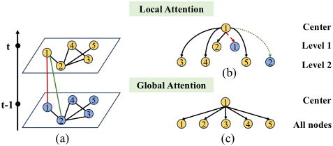
A simple way to learn high-order relationships from graphs is to apply self-attention Eq. 11, but it ignores the local hierarchical information. For example, the red dashed line and the green dotted line have different traffic propagation patterns and propagation time costs in Fig. 4(a) as a red dashed line only concerns the same node across different times, while a green dotted line concerns nodes at different space and times, which should not be ignored.
To fill this gap, we use a sub-tree structure that decouples the attention into multiple levels, as shown in Fig. 4(b). This structure enables fine-grained control over the contributions fromdifferent hopswithin the graph. In the sub-tree construction process, red dashed lines represent the formation of 1hop neighbours, while green dotted lines denote 2-hop neighbours. At each level k (k ∈ [1, K], where K denotes the number of levels), we compute the attention weights among the neighbours of a node n. These neighbours' representations are aggregated to obtain the localised representation hk,loc t,n , as formalised in Eq. 12. After computing hk,loc t,n for all nodes, the resulting vectors are assembled into the matrix Hk,loc t . Subsequently, we aggregate representations from all levels to form the final local attention Hloc t = ∑Kk=0 wkHk,loc t . Here, wk is a learnable parameter to control the contribution of each hop. This computation process can be seen as a khop message-passing process. Based on the k-hop messagepassing process, the maskMk in each step equals to A1 , denoted as A. Fig. 8(b) shows this matrix, where IN denotes an identity matrix of size N. Since the message-passing process runs for each edge and among all nodes, we obtain Hloc t with time complexity O(|E′ |). Here, E′ represents the number of edges after we build the edges across graphs from different time steps (i.e., number of 1's in A).
After obtaining Hloc t and Hglo t , we fuse them as follows:
where wglo is a learnable parameter. Then, we concatenate Ht from each time step t to obtain the output of the spatial self-attention layer H = ||Tt=0Ht.
We also use a temporal self-attention module to capture the temporal features from the full input time window. We merge Hsp with Hte to obtain the final output of each layer.
Discussion. The high-order and dynamic spatial-temporal relationships play an important role in traffic forecasting. Previous graph-based methods [Li and Zhu, 2021; Song et al., 2020] stack GNNs to capture such correlations, with suboptimal effectiveness, while the vanilla self-attention models suffer in their quadratic time complexity. Our work addresses these issues and presents a versatile self-attentionbased method to exploit the high-order and dynamic spatialtemporal relationships effectively and efficiently.
5 Experiments
5.1 Experimental Setup
Datasets. We use two freeway traffic datasets and an urban traffic dataset: PEMS03 and PEMS08 [PeMS, 2001] contain traffic flow data collected by 358 and 170 sensors on freeways in California; Melbourne [Su et al., 2024b] contains traffic flow data collected by 182 sensors in the City of Melbourne, Australia. The traffic records in PEMS03 and PEMS08 are given at 5-minute intervals (288 intervals per day), while those in Melbourne are given at 15-minute intervals (96 intervals per day). Melbourne has a higher standard deviation and is more challenging. See Table 3 (Appendix C.1 [Su et al., 2024a]) for the dataset statistics.
Following Li et al., we use records from the past hour to forecast for the next hour, i.e., T = T ′ = 1 hour in Eq. 1 over all datasets. We split each dataset into training, validation, and testing sets by 7:1:2 along the time axis.
Competitors. DualCast works with spatial-temporal models that follow the described self-attention-based structure. We implement DualCast with three such models: GMAN [Zheng et al., 2020], STTN [Xu et al., 2020], and PDFormer [Jiang et al., 2023a], denoted as DualCast-G, DualCast-S, and DualCast-P, respectively. We compare with the vanilla GMAN, STTN, and PDFormer models, plus GNN-based models GWNet [Wu et al., 2019], MTGNN [Wu et al., 2020], and STPGNN [Kong et al., 2024]. We further compare DualCast with MegaCRN [Jiang et al., 2023b] and EAST-Net [Wang et al., 2022], which focus on modelling non-stationarity in spatial-temporal series. We also compare with STWave [Fang et al., 2023] and STNorm [Deng et al., 2021], which consider disentanglement in forecasting.
| Model | PEMS03 | PEMS08 | Melbourne | |||
|---|---|---|---|---|---|---|
| RMSE↓ | MAE↓ | RMSE↓ | MAE↓ | RMSE↓ | MAE↓ | |
| GWNet MTGNN STPGNN MegaCRN EASTNet STNorm STWave STTN GMAN | 26.420±0.839 25.413±0.201 25.889±0.718 25.645±0.119 26.920±1.732 27.328±0.437 26.346±0.174 | 15.404±0.052 14.707±0.070 14.868±0.141 14.733±0.031 16.356±1.511 16.382±0.191 14.975±0.086 15.490±0.115 | 25.796±0.318 23.794±0.073 23.374±0.088 24.052±0.333 27.166±2.088 26.026±0.119 23.270±0.108 | 16.314±0.230 14.898±0.066 14.202±0.085 15.118±0.034 17.574±1.910 17.090±0.113 13.480±0.089 15.924±0.200 | 25.778±0.136 25.364±0.291 25.170±0.083 24.482±0.143 28.494±1.143 25.744±0.277 26.918±0.455 26.402±0.247 | 13.410±0.065 13.310±0.137 13.075±0.071 12.647±0.033 15.310±0.746 13.724±0.134 14.060±0.341 13.790±0.117 |
| DualCast-S (ours) DualCast-G (ours) | 25.582±0.414(+3.9%) | 15.370 ±0.086 (+0.8%) 15.094±0.099 (+2.7%) | 24.526±0.116 23.564±0.133 22.998±0.161 | 15.550±0.119 (+2.3%) 13.938±0.114 (+1.0%) 13.332±0.059 (+2.4%) | ||
| 27.166±0.408 | 24.984±0.248 | |||||
| 26.624±0.503 | 15.520±0.111 | 23.750±0.194 | 14.080±0.036 | 24.496±0.351 | 12.652±0.136 | |
| PDFormer | 25.950±0.421 | 14.690±0.080 | 23.250±0.099 | 13.654±0.337 | 27.072±0.301 | 14.230±0.069 |
| (ours) | 26.282±0.128 (+3.3%) | (+1.8%) (+0.8%) (+1.1%) | 25.474 ±0.184 (+3.5%) | 13.316±0.061 (+3.4%) | ||
| 23.978±0.105 (+2.1%) | 12.420±0.057 (+1.8%) | |||||
| DualCast-P | 24.898±0.663 (+4.1%) | 14.666±0.087 (+0.2%) | 26.040±0.150 (+3.8%) | 13.542±0.003 (+4.8%) | ||
| Error reduction | 2.0% | 0.2% | 1.1% | 1.1% | 2.1% | 1.8% |
Implementation details. We use the released code of the competitors, except for STTN which is implemented from Libcity [Wang et al., 2021]. We implement DualCast with the self-attention-based models following their source code, using PyTorch. We use the default settings from the source code for both the baseline models and their variants powered by DualCast. We train the models using Adam with a learning rate starting at 0.001, each in 100 epochs. For the models using DualCast, we use grid search on the validation sets to tune the hyper-parameters α, β, and γ. Table 4 (Appendix C.1 [Su et al., 2024a]) lists these hyper-parameter values. All experiments are run on an NVIDIA Tesla A100 GPU with 80 GB RAM. Following Xia et al., we use the average of root mean squared errors (RMSE) and mean absolute errors (MAE) for evaluation. Results are averaged over five runs.
5.2 Overall Results
Model performance across all times. Table 1 reports forecasting errors averaged over one hour. Powered by DualCast, DualCast-G, DualCast-P, and DualCast-S consistently outperform their vanilla counterparts. DualCast-P has the best performance on freeway traffic datasets PEMS03 and PEMS08, while DualCast-G performs the best on the urban traffic dataset Melbourne. Compared to PEMS03 and PEMS08, Melbourne represents an urban environment with greater variability in the traffic flow series (Table 3). GMAN's simple, robust design explains its strong performance in Melbourne, while PDFormer's reliance on time series clustering excels on PEMS03 and PEMS08 but struggles with Melbourne's variability, hindering cluster formation and accuracy. Fig. 5a further shows the RMSE for forecasting 15, 30, and 60 minutes forecasts, comparing DualCast-G, DualCast-P, and DualCast-S, their vanilla counterparts and top baselines MegaCRN and STPGNN. We see that the DualCast models outperform the baseline models consistently at different forecasting horizons, confirming their effectiveness. We also conducted t-tests and Wilcoxon tests over our model and the best baseline models across all datasets. We find that all results are statistically significant (with p ≪ 10-8 ).
Model performance during hours prone to traffic accidents. To verify DualCast's ability to learn complex environment contexts, we examine forecasting results during complex times (4:00 pm to 8:00 pm on workdays), which has reported a higher chance of traffic accidents [Karacasu et al., 2011; Ruikar, 2013]. Table 2 shows the results, where "all" means the RMSE at the 1-hour horizon for all days and "cpx" means that at complex times.
All models, including ours, have larger errors at complex times in most cases (except for STWave, GMAN, DualCastG, and DualCast-P on Melbourne), confirming it as a challenging period. Importantly, the errors of the DualCast-based models increase less at complex times compared to their vanilla counterparts. For example, the error gaps between DualCast-G and GMAN, and DualCast-P and PDFormer on PEMS08 double from 1.6% to 3.0% and 0.7% to 1.4%, respectively. Meanwhile, DualCast-P reduces the errors by up to 9.6% in Melbourne. These results confirm that disentangling intrinsic and environmental contexts improves forecast accuracy. Exceptions on Melbourne may arise due to its high data complexity, variance and skewness, making even a less complex time challenging.
5.3 Ablation Study
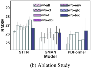
We implement six model variants: w/o-ct disables the CT attention from DualCast; w/o-f, w/o-dbi, and w/o-env remove the filter loss, the DBI loss, and the environment loss, respectively; w/o-glo and w/o-loc remove the global attention and local attention (including the CT attention), respectively.
As Fig. 5b shows, all DualCast modules enhance model performance. The DBI loss is more important on PEMS03, as PEMS03's freeway data exhibits clearer patterns across times and days, which DualCast can effectively learn with DBI loss guidance. More results are in Appendix C [Su et al., 2024a].
5.4 Parameter and Case study
Parameter study. We study the impact of α, β, and γ in our loss function (Eq. 10). Results confirm that DualCast is robust without the need for heavy tuning. More details are in Appendix C [Su et al., 2024a].
Case study. We conduct two case studies below.
Responding to traffic accidents. Cross-referencing Melbourne car crash reports [Victoria Road Crash Data, 2023] with the dataset revealed one accident during the data period. Fig. 5(c) compares 15-minute-ahead forecasts from
| Model | PEMS03 | PEMS08 | Melbourne | |||
|---|---|---|---|---|---|---|
| all | cpx | all | cpx | all | cpx | |
| GWNet | 30.152 | 37.276 | 29.162 | 31.986 | 27.766 | 29.186 |
| MTGNN | 27.984 | 34.842 | 26.253 | 28.616 | 27.264 | 27.994 |
| STPGNN | 29.405 | 35.346 | 26.095 | 27.320 | 27.018 | 27.510 |
| MegaCRN | 28.472 | 35.692 | 27.110 | 27.442 | 26.360 | 26.654 |
| EASTNet | 30.434 | 37.786 | 31.066 | 32.674 | 31.240 | 33.220 |
| ST-Norm | 30.895 | 38.956 | 29.366 | 31.948 | 27.752 | 29.304 |
| STWave | 29.210 | 37.312 | 25.600 | 27.130 | 29.562 | 29.324 |
| STTN | 30.386 | 40.990 | 28.182 | 31.400 | 29.108 | 30.554 |
| GMAN | 28.760 | 36.078 | 25.632 | 26.886 | 26.066 | 25.045 |
| PDFormer | 28.542 | 35.416 | 25.468 | 27.022 | 30.048 | 30.060 |
| DualCast-S (ours) | 29.494 (+2.9%) | 39.138 (+4.5%) | 27.522 (+2.3%) | 30.454 (+3.0%) | 27.256 (+6.4%) | 28.946 (+5.3%) |
| DualCast-G (ours) | 27.766 (+3.5%) | 34.450 (+4.5%) | 25.464 (+0.7%) | 26.506 (+1.4%) | 25.468 (+2.3%) | 24.398 (+2.6%) |
| DualCast-P (ours) | 27.542 (+3.5%) | 33.950 (+4.7%) | 25.048 (+1.6%) | 26.224 (+3.0%) | 28.134 (+6.4%) | 27.168 (+9.6%) |
| Error reduction | 1.6% | 2.6% | 1.7% | 2.5% | 2.3% | 2.6% |
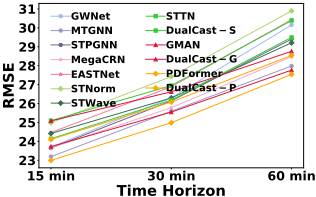
- (a) Forecasting error vs. time horizon
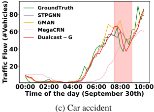
DualCast-G (best on this dataset), its vanilla counterpart GMAN, and the top-2 baselines (STPGNN, MegaCRN) at the sensor nearest the accident. Around 8:00, DualCast-G quickly captures the traffic change caused by the crash, producing forecasts closest to the ground truth.
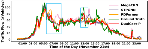
Responding to sudden changes in traffic. On the PEMS datasets, ground-truth traffic events are unavailable. Instead, we found two representative sensors (#72, see Appendix C.4 [Su et al., 2024a] and #97) on PEMS03 with sudden changes on November 21st, 2018. Fig. 6 shows the ground-truth traffic flow and 1-hour-ahead forecasts by MegaCRN, STPGNN, PDFormer, and DualCast-P at Sensor #97. DualCast-P closely aligns with the ground truth, especially during sudden changes, again highlighting the strength of DualCast. More results are in Appendix C [Su et al., 2024a], including PEMS08 and Melbourne results, an analysis of model scalability, effectiveness and potential for GNNbased models, and visualisations for disentangling results.
6 Conclusion
We proposed a framework named DualCast that enhances the robustness of self-attention-based traffic forecasting models, including the SOTA, in handling scenarios with complex environment contexts. DualCast takes a dual-branch structure to disentangle the impact of complex environment contexts, as guided by three loss functions. We further proposed a crosstime attention module to capture high-order spatial-temporal relationships. We performed experiments on real-world freeway and urban traffic datasets, where models powered by DualCast outperform their original versions by up to 9.6%. The best DualCast-based model outperforms the SOTA model by up to 2.6%, in terms of forecasting errors.
Ethical Statement
All datasets used in this study are publicly available and do not contain any personally identifiable information. There are no ethical concerns associated with this work.
Acknowledgments
This work is in part supported by the Australian Research Council (ARC) via Discovery Projects DP230101534 and DP240101006. Jianzhong Qi is supported by ARC Future Fellowship FT240100170. Feng Liu is supported by the ARC with grant numbers DE240101089, LP240100101, DP230101540 and the NSF&CSIRO Responsible AI program with grant number 2303037.
@inproceedings{ijcai2025p366,
  title     = {DualCast: A Model to Disentangle Aperiodic Events from Traffic Series},
  author    = {Su, Xinyu and Liu, Feng and Chang, Yanchuan and Tanin, Egemen and Sarvi, Majid and Qi, Jianzhong},
  booktitle = {Proceedings of the Thirty-Fourth International Joint Conference on
               Artificial Intelligence, {IJCAI-25}},
  publisher = {International Joint Conferences on Artificial Intelligence Organization},
  editor    = {James Kwok},
  pages     = {3290--3298},
  year      = {2025},
  month     = {8},
  note      = {Main Track},
  doi       = {10.24963/ijcai.2025/366},
  url       = {https://doi.org/10.24963/ijcai.2025/366},
}
TY - CPAPER TI - DualCast: A Model to Disentangle Aperiodic Events from Traffic Series AU - Su, Xinyu AU - Liu, Feng AU - Chang, Yanchuan AU - Tanin, Egemen AU - Sarvi, Majid AU - Qi, Jianzhong T2 - Proceedings of the Thirty-Fourth International Joint Conference on Artificial Intelligence, IJCAI-25 PB - International Joint Conferences on Artificial Intelligence Organization PY - 2025 SP - 3290 EP - 3298 DO - 10.24963/ijcai.2025/366 UR - https://doi.org/10.24963/ijcai.2025/366 ER -Copied
Machine-readable versions of this paper, for tools and AI agents:





