
ADFormer: Aggregation Differential Transformer for Passenger Demand Forecasting
Proceedings of the Thirty-Fourth International Joint Conference on Artificial Intelligence. Main Track. Pages 3353-3361.
https://doi.org/10.24963/ijcai.2025/373
Keywords
- Machine Learning: ML: Time series and data streams
- Machine Learning: ML: Attention models
- Data Mining: DM: Mining spatial and/or temporal data
- Data Mining: DM: Other
Abstract
Passenger demand forecasting helps optimize vehicle scheduling, thereby improving urban efficiency. Recently, attention-based methods have been used to adequately capture the dynamic nature of spatio-temporal data. However, existing methods that rely on heuristic masking strategies cannot fully adapt to the complex spatio-temporal correlations, hindering the model from focusing on the right context. These works also overlook the high-level correlations that exist in the real world. Effectively integrating these high-level correlations with the original correlations is crucial. To fill this gap, we propose the Aggregation Differential Transformer (ADFormer), which offers new insights to demand forecasting promotion. Specifically, we utilize Differential Attention to capture the original spatial correlations and achieve attention denoising. Meanwhile, we design distinct aggregation strategies based on the nature of space and time. Then, the original correlations are unified with the high-level correlations, enabling the model to capture holistic spatio-temporal relations. Experiments conducted on taxi and bike datasets confirm the effectiveness and efficiency of our model, demonstrating its practical value. The code is available at https://github.com/decisionintelligence/ADFormer.
- [Ba, 2016] Jimmy Lei Ba. Layer normalization. arXiv preprint arXiv:1607.06450, 2016.
- [Bai et al., 2020] Lei Bai, Lina Yao, Can Li, Xianzhi Wang, and Can Wang. Adaptive graph convolutional recurrent network for traffic forecasting. Advances in neural infor- mation processing systems, 33:17804-17815, 2020.
- [Berndt and Clifford, 1994] Donald J Berndt and James Clif- ford. Using dynamic time warping to find patterns in time series. In Proceedings of the 3rd international conference on knowledge discovery and data mining, pages 359-370, 1994.
- [Chen et al., 2018] Lu Chen, Qilu Zhong, Xiaokui Xiao, Yunjun Gao, Pengfei Jin, and Christian S Jensen. Price- and-time-aware dynamic ridesharing. In 2018 IEEE 34th international conference on data engineering, pages 1061-1072. IEEE, 2018.
- [di Torrepadula et al., 2024] Franca Rocco di Torrepadula, Enea Vincenzo Napolitano, Sergio Di Martino, and Nicola Mazzocca. Machine learning for public transportation de- mand prediction: A systematic literature review. Engineer- ing Applications of Artificial Intelligence, 137:109166, 2024.
- [Geng et al., 2019] Xu Geng, Yaguang Li, Leye Wang, Lingyu Zhang, Qiang Yang, Jieping Ye, and Yan Liu. Spatiotemporal multi-graph convolution network for ride- hailing demand forecasting. In Proceedings of the AAAI conference on artificial intelligence, volume 33, pages 3656-3663, 2019.
- [Guo et al., 2023] Shengnan Guo, Youfang Lin, Letian Gong, Chenyu Wang, Zeyu Zhou, Zekai Shen, Yiheng Huang, and Huaiyu Wan. Self-supervised spatial-temporal bottleneck attentive network for efficient long-term traffic forecasting. In 2023 IEEE 39th International Conference on Data Engineering, pages 1585-1596, 2023.
- [He et al., 2016] Kaiming He, Xiangyu Zhang, Shaoqing Ren, and Jian Sun. Deep residual learning for image recog- nition. In Proceedings of the IEEE conference on computer vision and pattern recognition, pages 770-778, 2016.
- [Hu et al., 2020] Jilin Hu, Bin Yang, Chenjuan Guo, Chris- tian S Jensen, and Hui Xiong. Stochastic origin- destination matrix forecasting using dual-stage graph con- volutional, recurrent neural networks. In 2020 IEEE 36th International conference on data engineering, pages 1417-1428. IEEE, 2020.
- [Huang et al., 2025] Yiheng Huang, Xiaowei Mao, Sheng- nan Guo, Yubin Chen, Junfeng Shen, Tiankuo Li, Youfang Lin, and Huaiyu Wan. Std-plm: Understanding both spa- tial and temporal properties of spatial-temporal data with plm. In Proceedings of the AAAI Conference on Artificial Intelligence, volume 39, pages 11817-11825, 2025.
- [Jiang et al., 2023] Jiawei Jiang, Chengkai Han, Wayne Xin Zhao, and Jingyuan Wang. Pdformer: Propagation delay- aware dynamic long-range transformer for traffic flow pre- diction. In Proceedings of the AAAI conference on artifi- cial intelligence, volume 37, pages 4365-4373, 2023.
- [Jin et al., 2022] Guangyin Jin, Zhexu Xi, Hengyu Sha, Yanghe Feng, and Jincai Huang. Deep multi-view graph- based network for citywide ride-hailing demand predic- tion. Neurocomputing, 510:79-94, 2022.
- [Ke et al., 2018] Jintao Ke, Hai Yang, Hongyu Zheng, Xiqun Chen, Yitian Jia, Pinghua Gong, and Jieping Ye. Hexagon- based convolutional neural network for supply-demand forecasting of ride-sourcing services. IEEE Transactions on Intelligent Transportation Systems, 20(11):4160-4173, 2018.
- [Li et al., 2024] Zhe Li, Xiangfei Qiu, Peng Chen, Yihang Wang, Hanyin Cheng, Yang Shu, Jilin Hu, Chenjuan Guo, Aoying Zhou, Qingsong Wen, et al. Foundts: Comprehen- sive and unified benchmarking of foundation models for time series forecasting. arXiv preprint arXiv:2410.11802, 2024.
- [Liang et al., 2024] Ruifeng Liang, Zhiheng Li, and Kai Zhang. Asstformer: Adaptive sparse spatial-temporal transformer for effective traffic forecasting. In 2024 5th International Seminar on Artificial Intelligence, Network- ing and Information Technology, pages 1847-1852, 2024.
- [Liu et al., 2023] Hangchen Liu, Zheng Dong, Renhe Jiang, Jiewen Deng, Jinliang Deng, Quanjun Chen, and Xuan Song. Spatio-temporal adaptive embedding makes vanilla transformer sota for traffic forecasting. In Proceedings of the 32nd ACM international conference on information and knowledge management, pages 4125-4129, 2023.
- [Lu et al., 2024] Jun Lu, Dan Wang, and Zhanquan Wang. Stpsformer: Spatial-temporal probsparse transformer for long-term traffic flow forecasting. In 2024 International Joint Conference on Neural Networks, pages 1-8, 2024.
- [Luo et al., 2023] Xunlian Luo, Chunjiang Zhu, Detian Zhang, and Qing Li. Stg4traffic: A survey and bench- mark of spatial-temporal graph neural networks for traffic prediction. CoRR, abs/2307.00495, 2023.
- [Pian et al., 2020] Weiguo Pian, Yingbo Wu, Xiangmou Qu, Junpeng Cai, and Ziyi Kou. Spatial-temporal dynamic graph attention networks for ride-hailing demand predic- tion. arXiv preprint arXiv:2006.05905, 2020.
- [Qiu et al., 2024] Xiangfei Qiu, Jilin Hu, Lekui Zhou, Xingjian Wu, Junyang Du, Buang Zhang, Chenjuan Guo, Aoying Zhou, Christian S Jensen, Zhenli Sheng, et al. Tfb: Towards comprehensive and fair benchmarking of time se- ries forecasting methods. Proceedings of the VLDB En- dowment, 17(9):2363-2377, 2024.
- [Qiu et al., 2025a] Xiangfei Qiu, Hanyin Cheng, Xingjian Wu, Jilin Hu, and Chenjuan Guo. A comprehensive sur- vey of deep learning for multivariate time series fore- casting: A channel strategy perspective. arXiv preprint arXiv:2502.10721, 2025. IJCAI
- [Qiu et al., 2025b] Xiangfei Qiu, Xingjian Wu, Yan Lin, Chenjuan Guo, Jilin Hu, and Bin Yang. Duet: Dual clus- tering enhanced multivariate time series forecasting. In SIGKDD, pages 1185-1196, 2025.
- [Shao et al., 2022] Zezhi Shao, Zhao Zhang, Fei Wang, Wei Wei, and Yongjun Xu. Spatial-temporal identity: A simple yet effective baseline for multivariate time series forecast- ing. In Proceedings of the 31st ACM International Con- ference on Information & Knowledge Management, pages 4454-4458, 2022.
- [Wu et al., 2019] Zonghan Wu, Shirui Pan, Guodong Long, Jing Jiang, and Chengqi Zhang. Graph wavenet for deep spatial-temporal graph modeling. In International Joint Conference on Artificial Intelligence 2019, pages 1907- 1913, 2019. IJCAI
- [Wu et al., 2020] Zonghan Wu, Shirui Pan, Guodong Long, Jing Jiang, Xiaojun Chang, and Chengqi Zhang. Con- necting the dots: Multivariate time series forecasting with graph neural networks. In Proceedings of the 26th ACM SIGKDD international conference on knowledge discov- ery & data mining, pages 753-763, 2020.
- [Wu et al., 2025] Xingjian Wu, Xiangfei Qiu, Zhengyu Li, Yihang Wang, Jilin Hu, Chenjuan Guo, Hui Xiong, and Bin Yang. Catch: Channel-aware multivariate time series anomaly detection via frequency patching. In ICLR, 2025.
- [Yan et al., 2021] Haoyang Yan, Xiaolei Ma, and Ziyuan Pu. Learning dynamic and hierarchical traffic spatiotemporal features with transformer. IEEE Transactions on Intelli- gent Transportation Systems, 23(11):22386-22399, 2021.
- [Yao et al., 2018] Huaxiu Yao, Fei Wu, Jintao Ke, Xianfeng Tang, Yitian Jia, Siyu Lu, Pinghua Gong, Jieping Ye, and Zhenhui Li. Deep multi-view spatial-temporal network for taxi demand prediction. In Proceedings of the AAAI con- ference on artificial intelligence, volume 32, pages 2588- 2595, 2018.
- [Ye et al., 2024] Tianzhu Ye, Li Dong, Yuqing Xia, Yutao Sun, Yi Zhu, Gao Huang, and Furu Wei. Differential trans- former. arXiv preprint arXiv:2410.05258, 2024.
- [Yu et al., 2022] Hongyuan Yu, Ting Li, Weichen Yu, Jian- guo Li, Yan Huang, Liang Wang, and Alex Liu. Regu- larized graph structure learning with semantic knowledge for multi-variates time-series forecasting. In International Joint Conference on Artificial Intelligence 2022, pages 2362-2368, 2022. IJCAI
- [Zhang et al., 2016] Junbo Zhang, Yu Zheng, Dekang Qi, Ruiyuan Li, and Xiuwen Yi. Dnn-based prediction model for spatio-temporal data. In Proceedings of the 24th ACM SIGSPATIAL international conference on advances in ge- ographic information systems, pages 1-4, 2016.
- [Zheng et al., 2020] Chuanpan Zheng, Xiaoliang Fan, Cheng Wang, and Jianzhong Qi. Gman: A graph multi- attention network for traffic prediction. In Proceedings of the AAAI conference on artificial intelligence, volume 34, pages 1234-1241, 2020.
- [Zheng et al., 2021] Bolong Zheng, Qi Hu, Lingfeng Ming, Jilin Hu, Lu Chen, Kai Zheng, and Christian S Jensen. Soup: Spatial-temporal demand forecasting and com- petitive supply in transportation. IEEE Transactions on Knowledge and Data Engineering, 35(2):2034-2047, 2021.
References were extracted automatically from the PDF and may contain errors.
Full text extracted automatically from the PDF; figures, tables and equations may differ. The PDF is the version of record.
1 Introduction
With the rise of digital and intelligent technologies, travel is becoming increasingly smart. Ride-hailing and bike-sharing services reflect this trend [Chen et al., 2018], but face inefficiencies like long wait times, vehicle idling, and unbalanced bicycle distribution. Accurate predictions are of great importance in real-world applications. [Luo et al., 2023] [Qiu et al., 2024] [Li et al., 2024] [di Torrepadula et al., 2024]
The key challenge in spatio-temporal data modeling lies in determining the appropriate structure to capture intricate
* Corresponding author: jlhu@dase.ecnu.edu.cn
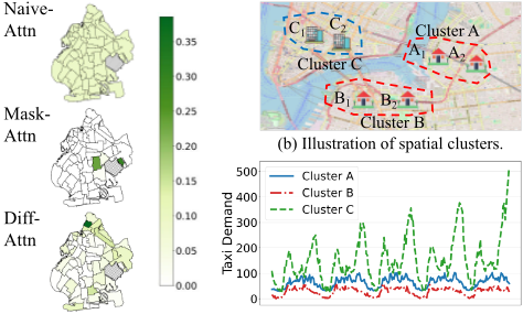
(a) Attention map of various methods.
(c) Demand trends of clusters.
Figure 1: Illustration of spatial attention noise and high-level correlations.
spatio-temporal dependencies. The topological relationships of cities describe the adjacency or containment relationships between regions, making spatio-temporal forecasting well suited for modeling with graph neural networks (GNNs). Consequently, GNNs have been widely applied in this field, such as [Geng et al., 2019] [Hu et al., 2020] [Zheng et al., 2021]. Next, with the success of attention models, some works argue that despite the notable success of GNN-based approaches, defining the adjacency matrix is challenging and they struggle to capture the dynamic nature of spatiotemporal data [Yan et al., 2021]. Therefore, recent studies [Jiang et al., 2023] [Lu et al., 2024] [Liang et al., 2024] adopted attention-based methods to address spatio-temporal problems, which can sufficiently understand the dynamics of spatial and temporal correlations. However, the attentionbased methods still suffer from the following drawbacks despite their effectiveness.
Firstly, the attention-based method tends to bring in attention noise that may disproportionately focus on irrelevant regions. As illustrated in Figure 1(a), we visualize the correlations between a specific region (shaded) and others under various methods. The observations are: 1) The naive attention mechanism exhibits dispersed relationships with generally low correlations across different regions. 2) The maskbased mechanism focuses only on local regions and few relevant areas. However, it is beneficial for us to concentrate on critical information, while most other areas maintain low correlations, as the bottom map depicts in Figure 1(a).
Secondly, current methodologies fail to adequately account for higher-level correlations from both spatial and temporal perspectives. For example, in Figure 1(b), the map depicts six distinct regions, where regions A1 and A2, as well as B1 and B2, represent residential areas, while C1 and C2 correspond to commercial areas. It is intuitive that regions in close geographical proximity exhibit similar dynamic patterns. Then, we aggregate regions A1 and A2 into a single entity, termed cluster A, and group B1 and B2 into cluster B, C1 and C2 into cluster C, we observe from Figure 1(c) that cluster A and cluster B exhibit similar demand patterns, while cluster C demonstrates distinct behavior. Thus, it is vital to consider higher-level correlations from the spatial perspective.
Further, strong temporal correlations must also be considered. For instance, taxi demand is typically high in residential areas and low in commercial areas during morning peak hours, while the reverse pattern occurs in afternoon peak hours. Furthermore, factors such as varying work schedules across companies lead to dynamic demand correlations over a broader time span. Existing approaches, such as those proposed by [Guo et al., 2023] and [Huang et al., 2025], incorporate reference point learning within attention mechanisms to capture high-order correlations. However, these methods are failing to adequately explore high-level temporal information. Additionally, they struggle to effectively integrate correlations from all sources, posing a challenge in accurate passenger demand forecasting.
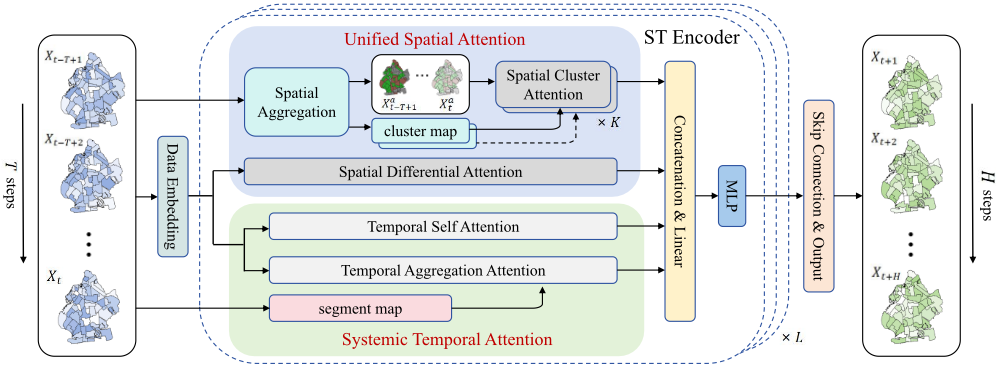
In this paper, we propose the Aggregation Differential Transformer (ADFormer) to effectively address the aforementioned challenges. To capture meaningful high-level spatial correlations, we introduce a Unified Spatial Attention module, which integrates Differential Attention to enhance spatial correlation detection while suppressing attention noise. We further apply spatial aggregation to identify and model high-level regional dependencies. For temporal modeling, we present a Systemic Temporal Attention module, consisting of temporal aggregation attention and selfattention blocks. The temporal aggregation employs a hierarchical temporal matrix, reconstructed via a learnable mapping from temporal information. In summary, the contributions of this paper are as follows:
- To reduce attention noise in spatial correlation detection, we apply Differential Attention to refine the attention matrix and enhance its robustness.
- To capture comprehensive spatio-temporal dependencies, we propose a region aggregation strategy that models non-pairwise spatial relationships while preserving original spatial correlations, along with a hierarchical temporal matrix to mitigate disruptions in temporal continuity caused by irregular time intervals.
- Extensive experiments conducted on three real-world datasets from two cities demonstrate that our proposed model, ADFormer, surpasses state-of-the-art baselines in forecasting accuracy while maintaining computational efficiency, highlighting its practical applicability.
2 Preliminaries
2.1 Notations and Definitions
Definition 1 (Urban Region). An urban region corresponds to a boundary, such as a zone, within the real world context, denoted as r. The area of interest can be partitioned into a set of non-overlapping regions, denoted as R = {r1, r2, . . . , rN}, where N is the total number of urban regions.
Definition 2 (Spatial Cluster). A spatial cluster is defined as a set of urban regions aggregated based on a specific aggregation criterion, denoted as C = {r1, r2, . . . , r|C|}. For instance, if the aggregation criterion is functional similarity, the regions within a cluster share similar functionalities. Under this criterion, the area of interest can be partitioned into a set of disjoint clusters, represented as C = {C1,C2, . . . ,CM}, where M is the total number of clusters.
Definition 3 (Region Passenger Demand). Passenger demand is defined as the total number of passengers requesting service within a region at a specific time step t, denoted as xt ∈ RD , where D represents the dimensionality of the features. The passenger demand across an urban region over the past T time steps is represented as Xraw ∈ RT×N×D .
2.2 Problem Statement
Given historical observation data [Xraw t-T+1 , . . . ,X raw t ], our goal is to learn a mapping function f(·) that can generate accurate predictions for future demand, which can be formulated as follows.
where T represents the historical window and H denotes the future horizon.
3 Methodology
In this section, we first introduce how to embed the data into the high-dimensional space. Then, we explain how to capture their original correlations and high-level correlations from spatial and temporal perspectives, respectively. Finally, we describe the way to fuse them in the output layer. The overall framework is presented in Figure 2.
3.1 Data Embedding
To improve the model's ability to capture the periodic patterns inherent in passenger demand, we augment the original data with time-related features. These features include the time of day and the day of the week, which reflect the significant periodicity in passenger demand:
where ∥ denotes the concatenation operator and Xfull ∈ RT×N×D′ . Td ∈ RT×N×1 represents the time of day and Tw ∈ RT×N×7 is the one-hot vector of the day of week.
Then, fully connected layers are used to map Xraw and the additional time-related information to high-dimensional space separately, and subsequently sum them together:
where Xemb ∈ RT×N×d . Wraw ∈ RD×d ,WTd ∈ R1×d and WTw ∈ R7×d are learnable parameters.
Since the self-attention mechanism does not inherently contain sequential information, we adopt the classical positional encoding scheme, leveraging the periodicity of sine and cosine functions to generate positional information for the input sequence, namely Xpos ∈ RT×d .
Furthermore, regions have distinct roles in a city and their passenger demand patterns vary accordingly. Inspired by [Shao et al., 2022], a simple yet effective model, we introduce a spatial embedding Xspa ∈ RN×d as an identifier for each region. Finally, all components are summed and used as the subsequent input:
X will be used to replace Xinput for convenience in the following text.
3.2 Unified Spatial Attention
To consider spatial correlations of both urban regions and spatial clusters, we propose a unified spatial attention module that consists of 1) Spatial Differential Attention and 2) Spatial Cluster Attention, which are detailed as follows.
Spatial Differential Attention
To address the issue of attention noise in spatial correlations at the urban region level, we examine the limitations of the original attention mechanism. It has been demonstrated that the original attention mechanism tends to over-attend to irrelevant context, a phenomenon that is particularly pronounced in spatial attention applications, especially when considering urban regions where a larger number of elements are involved in the attention computation. To mitigate this issue, we apply the recently proposed differential attention mechanism, as introduced in large language model studies [Ye et al., 2024], to the spatio-temporal data domain. Following the structure of the differential attention mechanism, we first compute the Query, Key, and Value matrices as outlined below:
where W S Q , W SK , W S V ∈ Rd×ds1 are learnable parameters. QS1 , QS2 , KS 1 ,KS 2 ∈ RT×N×(ds1 /2) are the queries and keys of the computation of two attention score matrices. V S ∈ RT×N×ds1 is the value of the differential attention operation.
Then, we can obtain the spatial output at the urban region level based on the differential attention as follows:
where λ is a learnable scalar. The result of the difference of the two attention matrices represents the denoised attention scores among the N regions. Aligned with [Ye et al., 2024], we set the scalar λ as:
where λq1 , λk1 , λq2 and λk2 ∈ Rds1 /2 are learnable vectors. λinit is a randomly initialized constant.
Spatial Cluster Attention
To capture high-level correlations among regions, we aggregate them based on the similarity of their historical demand data, which reflects their functional roles within the urban environment. This approach groups regions with similar demand patterns, even if they are geographically distant. For instance, two commercial centers located far apart may exhibit comparable trends due to similar functions. Such aggregation enables the model to capture functional similarities beyond spatial proximity.
Specifically, we calculate the similarity of historical data between two regions through the Dynamic Time Warping (DTW) [Berndt and Clifford, 1994] algorithm, further attaining the distance matrix Msim ∈ RN×N , which describes the similarity distances between regions.
Regions are aggregated based on Msim. Initially, each region is considered as a separate cluster. Then, calculate distances between clusters:
where Ci = {r1, . . . , r|Ci|} and Cj = {r1′ , . . . , r|Cj|}. Iteratively merge the closest clusters until the desired number of clusters is achieved, resulting in the final clustering C.
For aggregated clusters, we adjust the cluster sizes to ensure that the aggregation results are balanced to some extent. For instance, move region p to Cj if the size of the cluster to which p belongs exceeds the threshold and the distance to the cluster Cj is the smallest.
In this way, we can identify which original regions are included in the clusters, helping us to get the cluster map, denoted Mcls ∈ RM×N . Based on this, we aggregate the Xraw to obtain Xagg:Xagg = MclsXraw ∥ Td ∥ Tw. (9)
Xagg eventually becomes Xemb agg ∈ RT×M×d via Data Embedding with temporal information enhancement and spatial identity assignment. We will use Xa to replace Xemb agg for convenience. Next, we employ spatial cluster self-attention (SCA) to model the high-level correlations:
where W C Q ,W C K , W C V ∈ Rd×ds2 are learnable mapping matrices. After capturing the high-level correlations, we need to map these back to the original spatial level to assist in forecasting the demand volume in the regions. We take advantage of the Mcls to help initialize the learnable separation parameter, aiming to allocate the correlations of clusters to regions that are closely related to them:
where ⊙ represents Hadamard product and Msep ∈ RM×N is a randomly initialized parameter.
3.3 Systemic Temporal Attention
Temporal correlation is another important aspect of passenger demand forecasting, which also involves multi-level correlations. Thus, we propose a Systemic Temporal Attention module, which is shown in Figure 3. This module consists of a) Temporal Self Attention and b) Temporal Aggregation Attention to capture the multi-level temporal correlations. It is worth mentioning that, due to the relatively few time steps in passenger demand forecasting, we do not use Differential Attention to denoise attention along the temporal dimension.
Temporal Self Attention
We make use of the self-attention mechanism to extract temporal correlations among regions. Firstly, we transpose X to XT ∈ RN×T×d and map it to query, key and value:
……
……
- (a) Temporal Self Attention.
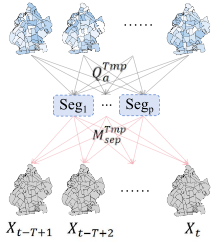
Figure 3: Systemic Temporal Attention.
where W Tmp Q ,W Tmp K ,W Tmp V ∈ Rd×dt1 are learnable mapping parameters.
Then, we compute the attention scores to obtain the correlations between time steps, thereby deriving the output of temporal self attention:
where ATmp = QTmp (KTmp )T √dt1 ∈ RN×T×T represents the correlations between steps among regions.
Temporal Aggregation Attention
Similar to spatial aggregation, it is also difficult to obtain an explicit aggregation in passenger demand forecasting. In this paper, we employ a learnable matrix QTmp a ∈ RN×P×dt2 to act as the query during the calculation of attention:
where W Tmpa K ,W Tmpa V ∈ Rd×dt2 are mapping parameters. We leverage temporal information within the data to derive the restoration matrix M Tmp sep ∈ RN×T×P :
where (Xfull[:, :,D : D′ ])T ∈ RN×T×(D′-D) and Wsep ∈ R(D′-D)×P is a learnable parameter.
3.4 Output Layer
Attention Fusion
We need to integrate the attention mechanisms applied in multiple aspects. For spatial dimension, we perform multilevel spatial aggregations in the encoder of each layer, namely Xa = {Xa1 , . . . ,XaK }. Accordingly, K calculations of SCA(Xai ) are required. Overall, spatial attention (SA) can be formally expressed as:
where ∥ denotes concatenation and each aggregation level has an associated cluster map in spatial cluster attention.
In terms of temporal dimension, we use only one aggregation per layer to reduce complexity. Temporal attention (TA) can be expressed in a formulated way:
Spatial-Temporal Encoder
After merging the spatial and temporal attention at each level respectively, we integrate all components globally and perform forward propagation via fully connected layers:
where W O ∈ R(ds1+ds2+dt1+dt2 )×d is a learnable projection parameter. We stack L encoder layers to obtain the final output and utilize layer normalization [Ba, 2016] and residual connection [He et al., 2016] to stabilize the training process.
4 Experiments
4.1 Experimental Settings
Datasets
We evaluate our model on three widely used public datasets: NYC-Taxi 1 , NYC-Bike 2 , and Xi'an-Taxi, which exhibit diverse urban structures and demand distributions. NYCTaxi/Bike. These two datasets record transportation activity across 263 boroughs (i.e., urban regions) in New York. Each taxi or bike trip includes information such as start/end time, locations, cost, and other details. Based on pickup and drop-off times, we record the number of passengers or rides in 30-minute intervals. The NYC-Taxi data spans January-December 2016, while the NYC-Bike data covers the same period in 2023. Xi'an-Taxi. This dataset, provided by Didi, a ride-hailing company in China, contains vehicle trajectories during passenger trips. Each trajectory includes timestamps and GPS coordinates. We extract trip origin points and divide the city into non-overlapping hexagonal grids to generate demand sequences. The data spans October and November 2016.
For each dataset, we split the data into training, validation, and test sets in a 7:1:2 ratio. For single-step prediction, the past three hours (6 steps) of demand data are used to forecast the next 30 minutes (1 step). For multi-step prediction, the same input is used to predict demand over the next 1.5 hours (3 steps) and 3 hours (6 steps).
Baselines
We compare ADFormer with seven baselines across two categories. (1) GCN-based models. GWNet [Wu et al., 2019], MTGNN [Wu et al., 2020], AGCRN [Bai et al., 2020], RGSL [Yu et al., 2022]. (2) Attention-based models. GMAN [Zheng et al., 2020], PDFormer [Jiang et al., 2023], ASSTFormer [Liang et al., 2024].
1 https://www.nyc.gov/site/tlc/about/tlc-trip-record-data.page
2 https://citibikenyc.com/system-data
Model Parameters
The experimental environment is configured as follows: the Python version is 3.10.0, the CUDA version is 12.1, and the PyTorch version is 2.5.1. We conduct experiments on an NVIDIA GeForce RTX 3090 with 24GB of memory. The AdamW optimizer is used in model training, with an initial learning rate of 1e-3, decaying to 1e-4. We explore hidden dimension ∈ {32, 64, 128}, the depth of encoder ∈ {4, 6, 8} and impact of number of spatial clusters and hierarchical levels in the Parameter Study.
Metrics
We take Mean Absolute Error (MAE), Root Mean Squared Error (RMSE) and Mean Absolute Percentage Error (MAPE) as evaluation metrics. Following [Yao et al., 2018], we exclude steps with low demand and set the threshold to 5, which means that points less than the value are not considered.
4.2 Overall Performance
As shown in Table 1, our model consistently outperforms baselines, demonstrating strong performance in real-world demand forecasting. Among dynamic graph methods, the performance is similar due to shared message-passing mechanisms. MTGNN stands out by jointly modeling time series and learning graph structures.
Attention-based methods generally outperform graphbased ones by better capturing dynamic correlations. PDFormer stands out for its ability to model spatio-temporal dynamics during attention computation and filter out lowrelevance pairs, leading to improved performance. ASSTFormer performs well on datasets with fewer regions, such as Xi'an Taxi, but as the number of regions increases, its topk strategy struggles to capture complex correlations, resulting in performance degradation.
Compared to the above baselines, our model takes into account the high-level correlations in both spatial and temporal aspects of spatio-temporal data, leading to a more comprehensive modeling of spatio-temporal correlations. In addition, by incorporating the differential attention mechanism, we selectively amplify the most informative correlations while suppressing noise. These factors contribute to the superior performance of our model.
Beyond that, our method's extensive capture of high-level correlations might intuitively suggest a slower runtime. In PDFormer, this approach achieves a balance between performance and efficiency, excelling in both aspects. Therefore, we compared the runtimes of the two methods through multistep forecasting experiments. As shown in Table 2, the results demonstrate that our model is fast in both training and inference due to Flash-Attn support, validating our model's practical value.
4.3 Ablation Study
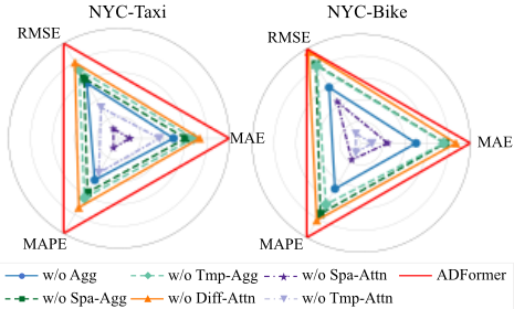
We further validate the role of each module in the model by removing certain modules from our model. (1) w/o Diff-Attn removes the differential attention mechanism in spatial correlations modeling. (2) w/o Agg ignores the high-level spatiotemporal correlations, with the model only capturing correlations within the data at the original level. (3) w/o Spa-Agg removes spatial aggregation and focuses solely on temporal aggregation. (4) w/o Tmp-Agg considers only spatial aggregation. (5) w/o Spa-Attn only captures correlations in the temporal aspect. (6) w/o Tmp-Attn only captures correlations in spatial aspect. We conduct multi-step prediction experiments on the NYC datasets. The experimental results are inverted and normalized to facilitate visualization, as shown in Figure 4. In the figure, lines closer to the outer edges indicate better performance. We draw the following conclusions:
| Dataset | Horizon | Metric | GWNet | MTGNN | AGCRN | RGSL | GMAN | PDFormer | ASSTFormer | ADFormer |
|---|---|---|---|---|---|---|---|---|---|---|
| NYC Taxi | MAE RMSE | 5.697 11.871 18.919 | 5.677 11.833 18.718 | 5.797 13.304 18.768 | 5.724 12.555 18.677 | 5.662 11.750 19.081 | 5.625 11.597 18.920 | 5.756 11.953 19.185 | 5.461 11.342 18.238 | |
| 30 min 90 min | MAPE MAE RMSE MAPE | 6.344 13.687 20.237 | 6.229 13.532 19.758 | 6.486 14.600 20.171 | 6.388 14.327 20.027 | 6.273 13.565 20.134 | 6.131 13.128 21.036 | 6.358 13.807 21.422 | 5.975 12.920 20.348 | |
| 3 hour | MAE RMSE MAPE | 6.922 15.363 21.303 | 6.809 15.158 21.162 3.405 | 6.979 16.222 21.406 3.401 5.381 | 7.052 16.133 21.704 3.371 | 6.897 15.397 21.785 | 6.684 14.776 21.129 | 7.053 22.244 3.463 5.409 | 6.543 | |
| NYC Bike | 30 min 90 min | MAE RMSE MAPE MAE | 5.569 25.531 3.899 | 5.348 25.009 3.731 | 25.044 3.727 6.059 | 5.289 24.977 3.674 | 3.416 5.321 25.323 3.765 | 5.230 25.251 | 3.799 6.211 | 3.299 5.104 24.585 |
| RMSE MAPE | 6.433 28.529 | 6.016 27.381 | 27.657 | 5.943 27.248 4.176 | 6.073 27.858 4.271 | 3.741 5.973 27.499 | 28.084 | 3.588 5.731 26.664 | ||
| 3 hour | MAE RMSE MAPE | 4.481 7.685 32.909 | 4.179 7.011 31.856 | 4.212 7.029 32.528 | 7.065 32.054 | 7.227 31.964 | 4.215 7.107 | 4.167 7.038 | 4.029 6.810 31.563 | |
| 30 min | MAE RMSE MAPE | 3.623 5.312 | 3.684 5.553 | 3.702 5.503 22.502 | 3.812 5.576 24.037 | 32.635 3.741 | 3.696 | 3.564 5.208 22.848 | ||
| Xi'an | 90 min | MAPE | 3.493 | 3.804 5.663 | 22.353 | 3.845 5.768 | 5.902 24.216 | 3.397 | 16.135 | 14.592 20.619 |
| MAE RMSE | 22.159 | 4.046 | 4.146 | 25.808 | ||||||
| 23.195 | 5.453 24.098 | |||||||||
| 3.671 | 3.843 | 5.727 | ||||||||
| 4.011 | 3.959 | 5.794 23.168 | 4.074 | 4.034 | 22.464 3.830 | |||||
| RMSE | 5.693 23.504 | 3.961 | 6.159 | 6.228 | 23.660 | 5.466 | ||||
| 5.357 22.631 | 32.754 | |||||||||
| Taxi | 3.852 | 3.973 | 3.697 | |||||||
| MAE | 5.415 | |||||||||
| 23.487 | ||||||||||
| 3.887 | 3.865 5.735 | |||||||||
| 23.107 | 23.232 | |||||||||
| 3 hour | MAPE | 24.229 | 5.976 | 6.061 | 5.706 | |||||
| 6.003 | 5.959 | 6.061 | 23.114 | |||||||
| 23.778 | 23.826 | |||||||||
| 23.822 | 24.168 | 24.723 | 24.589 |
| Dataset | Phase | PDFormer | ADFormer |
|---|---|---|---|
| NYC-Taxi | training inference | 53.75 2.89 | 35.51 1.68 |
| NYC-Bike | training inference | 48.17 2.12 | 25.62 1.18 |
- Capturing correlations from only spatial or temporal perspective is insufficient. As indicated by the dark and light purple dashed lines in the figure, spatial correlations are indispensable for taxi demand, while temporal correlations are pivotal for bike demand. This may be because taxi rides generally cover a larger spatial range and are more closely related to the functionality of dissimilar regions, whereas bike usage is more time sensitive.
- Spatio-temporal aggregation is essential for modeling data correlations, as relying solely on temporal or spatial aggregation is limited. As shown by the dark and light green dashed lines, the relative importance of each varies: spatial aggregation is more impactful in the taxi dataset, while in the bike dataset, temporal aggregation plays a greater role. This aligns with the pattern observed at the first point.
- The Differential Attention mechanism is particularly effective in spatially dominant scenarios like taxi demand, but less effective when temporal dependencies, such as those in bike demand, play a more significant role. This is mainly because it is applied only along the spatial dimension, given the relatively short temporal sequence length in our setting.
4.4 Parameter Study
To investigate the impact of the number of spatial clusters on the experimental results, we design a parameter study from the perspectives of both hierarchy and quantity on the Xi'anTaxi dataset for single-step and multi-step forecasting tasks, while NYC datasets yield similar results. We first test a spatial aggregation-free architecture, followed by architectures with one-level, two-level, and three-level spatial aggregation, as shown in Table 3. The results lead to two key conclusions:
[64,8] [96,16,8]
3.694
5.457
22.402
3.814
5.689
23.039
| Xi'an | Horizon | Metric | w/o spa-agg 3.782 | [16] | [64] | [64,16] | [64,8] |
|---|---|---|---|---|---|---|---|
| 90 min | MAE | 3.713 | 3.719 | 3.697 | 3.705 | ||
| RMSE | 5.601 | 5.488 | 5.511 | 5.466 | 5.488 | ||
| MAPE | 22.824 | 22.525 | 22.540 | 22.465 | 22.454 | ||
| Taxi | 3 | MAE | 3.935 | 3.875 | 3.849 | 3.830 | 3.836 |
| hour | RMSE | 5.880 | 5.786 | 5.744 | 5.706 | 5.727 | |
| MAPE | 23.658 | 23.291 | 23.147 | 23.114 | 23.093 |
- Forecasting accuracy improves regardless of the number of aggregation levels. And performance tends to enhance as the number of levels increases.
- The benefit of deeper aggregation levels becomes more pronounced at longer forecasting horizons, as high-level spatial correlations generally unfold over extended time spans, consistent with the temporal dynamics of human mobility between functional zones.
Notably, the results suggest that our model exhibits robustness with respect to this parameter. In practice, prior knowledge of functional zone categorizations within a city or specific regions can provide valuable guidance for parameter configuration.
4.5 Case Study
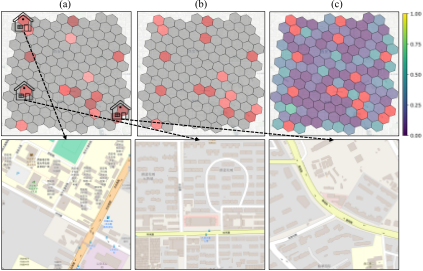
We visualize the high-level spatial correlations learned by our model to better illustrate the effectiveness of our approach. As illustrated in Figure 5, the urban area in the Xi'an dataset is divided into hexagonal grids. In (a), there are six clusters filled with dark or light red. In reality, these grids mostly contain residential areas. The second row of maps displays three grids that are relatively similar. These grids not only contain a large number of residential areas, but also include major intersections, indicating their spatial similarity and the potential for aggregation. Subfigure (b) shows larger clusters that are formed by aggregating the smaller clusters in (a), incorporating more regions. Finally, subfigure (c) presents the aggregation results at the highest level and illustrates the relationships between clusters, where grids of the same color belong to the same cluster. The core idea of spatial aggregation is to break artificially defined spatial boundaries and view spatial correlations from a holistic perspective. The concept of temporal aggregation is similar to this.
5 RelatedWorks
Early works [Zhang et al., 2016; Yao et al., 2018; Ke et al., 2018] widely adopted Convolutional Neural Networks (CNNs), modeling urban regions as grids with each area represented as a pixel, and using CNNs to capture spatiotemporal dependencies. However, geospatial data has inherent topological characteristics, such as spatial irregularity and local perception, which make Graph Neural Networks (GNNs) more suitable than CNNs for modeling these structures. For example, [Geng et al., 2019] integrates non-Euclidean pairwise correlations among regions through multi-graph convolution. [Pian et al., 2020] uses an attention mechanism to assign importance to neighboring regions and builds a dynamic graph to capture time-specific spatial relationships. [Jin et al., 2022] integrates 1D CNNs and multi-graph attention networks to capture short-term spatial and long-term temporal dynamics. While graph structures intuitively model spatial connections, defining adjacency matrices that accurately reflect spatial dynamics remains challenging.
To better tackle this issue, several attention-based spatiotemporal prediction models have been proposed. These models aim to learn spatio-temporal dynamics directly from the data rather than pre-defining the graph structure. For instance, [Yan et al., 2021] uses a K-hop adjacent mask to allow the model to focus on local information. [Jiang et al., 2023] incorporates two masking matrices in spatial self-attention to capture both short-range spatial correlations based on distance and long-range correlations based on historical data similarity. [Liang et al., 2024] applies a self-corrected top-K mechanism to filter attention scores, achieving attention denoising. Meanwhile, recent methods focus on processing input data, such as incorporating adaptive embeddings and decomposing from the perspective of channel or variables [Liu et al., 2023] [Qiu et al., 2025b] [Wu et al., 2025] [Qiu et al., 2025a]. However, these models often overemphasize correlations between unrelated objects, limiting their ability to focus on more relevant spatio-temporal relations. In this paper, we propose a method to reduce attention noise from unrelated regions while reinforcing the connections between related regions and consider holistic spatio-temporal correlations, thereby improving spatio-temporal forecasting accuracy.
6 Conclusion
In this work, we propose the Aggregation Differential Transformer (ADFormer) for passenger demand forecasting. ADFormer integrates Differential Attention to denoise raw spatial correlations and adopts a region aggregation strategy to capture high-level, non-pairwise spatial dependencies. Additionally, a hierarchical temporal matrix approach is developed to model broader and more intricate temporal dependencies. The effectiveness of ADFormer is evaluated on public datasets, including ablation studies that validate the contributions of the aggregation strategies and Differential Attention. Our findings reveal that the influence of temporal and spatial correlations varies across different scenarios, reflecting the inherent nature of the datasets. Furthermore, the parameter study and the case study quantitatively and qualitatively demonstrate the effectiveness of spatial aggregation.
Acknowledgements
This work was partially supported by National Natural Science Foundation of China (62472174). This work was supported by "the Open Research Fund of Key Laboratory of Advanced Theory and Application in Statistics and Data Science-MOE,ECNU". Jilin Hu is the corresponding author of the work.
@inproceedings{ijcai2025p373,
  title     = {ADFormer: Aggregation Differential Transformer for Passenger Demand Forecasting},
  author    = {Wang, Haichen and Yang, Liu and Zhang, Xinyuan and Yu, Haomin and Li, Ming and Hu, Jilin},
  booktitle = {Proceedings of the Thirty-Fourth International Joint Conference on
               Artificial Intelligence, {IJCAI-25}},
  publisher = {International Joint Conferences on Artificial Intelligence Organization},
  editor    = {James Kwok},
  pages     = {3353--3361},
  year      = {2025},
  month     = {8},
  note      = {Main Track},
  doi       = {10.24963/ijcai.2025/373},
  url       = {https://doi.org/10.24963/ijcai.2025/373},
}
TY - CPAPER TI - ADFormer: Aggregation Differential Transformer for Passenger Demand Forecasting AU - Wang, Haichen AU - Yang, Liu AU - Zhang, Xinyuan AU - Yu, Haomin AU - Li, Ming AU - Hu, Jilin T2 - Proceedings of the Thirty-Fourth International Joint Conference on Artificial Intelligence, IJCAI-25 PB - International Joint Conferences on Artificial Intelligence Organization PY - 2025 SP - 3353 EP - 3361 DO - 10.24963/ijcai.2025/373 UR - https://doi.org/10.24963/ijcai.2025/373 ER -Copied
Machine-readable versions of this paper, for tools and AI agents:





