
FreqLLM: Frequency-Aware Large Language Models for Time Series Forecasting
Proceedings of the Thirty-Fourth International Joint Conference on Artificial Intelligence. Main Track. Pages 3389-3397.
https://doi.org/10.24963/ijcai.2025/377
Keywords
- Machine Learning: ML: Regression
- Machine Learning: ML: Time series and data streams
- Data Mining: DM: Mining spatial and/or temporal data
Abstract
Large Language Models (LLMs) have recently shown promise in Time Series Forecasting (TSF) by effectively capturing intricate time-domain dependencies. However, our preliminary experiments reveal that standard LLM-based approaches often fail to capture global correlations, limiting predictive performance. We found that embedding frequency-domain signals smooths weight distributions and enhances structured correlations by clearly separating global trends (low-frequency components) from local variations (high-frequency components). Building on these insights, we propose FreqLLM, a novel framework that integrates frequency-domain semantic alignment into LLMs to refine prompts for improved time series analysis. By bridging the gap between frequency signals and textual embeddings, FreqLLM effectively captures multi-scale temporal patterns and provides more robust forecasting results. Extensive experiments on benchmark datasets demonstrate that FreqLLM outperforms state-of-the-art TSF methods in both accuracy and generalization. The code is available at https://github.com/biya0105/FreqLLM.
- [Ariyo et al., 2014] Adebiyi A Ariyo, Adewumi O Adewumi, and Charles K Ayo. Stock price predic- tion using the arima model. In 2014 UKSim-AMSS 16th international conference on computer modelling and simulation, pages 106-112. IEEE, 2014.
- [Chen et al., 2021] Qiwei Chen, Changhua Pei, Shanshan Lv, Chao Li, Junfeng Ge, and Wenwu Ou. End-to-end user behavior retrieval in click-through rateprediction model. arXiv preprint arXiv:2108.04468, 2021.
- [Cui et al., 2024] Can Cui, Yunsheng Ma, Xu Cao, Wenqian Ye, Yang Zhou, Kaizhao Liang, Jintai Chen, Juanwu Lu, Zichong Yang, Kuei-Da Liao, et al. A survey on multi- modal large language models for autonomous driving. In Proceedings of the IEEE/CVF Winter Conference on Ap- plications of Computer Vision, pages 958-979, 2024.
- [Das et al., 2023] Abhimanyu Das, Weihao Kong, Andrew Leach, Shaan Mathur, Rajat Sen, and Rose Yu. Long-term forecasting with tide: Time-series dense encoder. Trans. Mach. Learn. Res., 2023, 2023.
- [Dimri et al., 2020] Tripti Dimri, Shamshad Ahmad, and Mohammad Sharif. Time series analysis of climate vari- ables using seasonal arima approach. Journal of Earth Sys- tem Science, 129:1-16, 2020.
- [Ghosal et al., 2023] Deepanway Ghosal, Navonil Ma- jumder, Ambuj Mehrish, and Soujanya Poria. Text-to- audio generation using instruction-tuned llm and latent diffusion model. arXiv preprint arXiv:2304.13731, 2023.
- [Gruver et al., 2024] Nate Gruver, Marc Finzi, Shikai Qiu, and Andrew G Wilson. Large language models are zero- shot time series forecasters. Advances in Neural Informa- tion Processing Systems, 36, 2024.
- [He et al., 2022a] Hui He, Qi Zhang, Simeng Bai, Kun Yi, and Zhendong Niu. Catn: Cross attentive tree-aware net- work for multivariate time series forecasting. In Proceed- ings of the AAAI Conference on Artificial Intelligence, vol- ume 36, pages 4030-4038, 2022.
- [He et al., 2022b] Kaiming He, Xinlei Chen, Saining Xie, Yanghao Li, Piotr Dollár, and Ross Girshick. Masked au- toencoders are scalable vision learners. In Proceedings of the IEEE/CVF conference on computer vision and pattern recognition, pages 16000-16009, 2022.
- [Jin et al., 2024] Ming Jin, Shiyu Wang, Lintao Ma, Zhixuan Chu, James Zhang, Xiaoming Shi, Pin-Yu Chen, Yuxuan Liang, Yuan-fang Li, Shirui Pan, et al. Time-llm: Time se- ries forecasting by reprogramming large language models. In International Conference on Learning Representations, 2024.
- [Kim et al., 2021] Taesung Kim, Jinhee Kim, Yunwon Tae, Cheonbok Park, Jang-Ho Choi, and Jaegul Choo. Re- versible instance normalization for accurate time-series forecasting against distribution shift. In International Con- ference on Learning Representations, 2021.
- [Kinga et al., 2015] D Kinga, Jimmy Ba Adam, et al. A method for stochastic optimization. In International con- ference on learning representations (ICLR), volume 5, page 6. San Diego, California;, 2015.
- [Koprinska et al., 2018] Irena Koprinska, Dengsong Wu, and Zheng Wang. Convolutional neural networks for en- ergy time series forecasting. In 2018 international joint conference on neural networks (IJCNN), pages 1-8. IEEE, 2018.
- [Liang et al., 2024] Yuxuan Liang, Haomin Wen, Yuqi Nie, Yushan Jiang, Ming Jin, Dongjin Song, Shirui Pan, and Qingsong Wen. Foundation models for time series anal- ysis: A tutorial and survey. In Proceedings of the 30th ACM SIGKDD conference on knowledge discovery and data mining, pages 6555-6565, 2024.
- [Lin et al., 2024] Shengsheng Lin, Weiwei Lin, Wentai Wu, Songbo Wang, and Yongxiang Wang. Petformer: Long- term time series forecasting via placeholder-enhanced transformer. IEEE Transactions on Emerging Topics in Computational Intelligence, 2024.
- [Liu and Chen, 2024] Jiexi Liu and Songcan Chen. Timesurl: Self-supervised contrastive learning for universal time series representation learning. In Proceed- ings of the AAAI Conference on Artificial Intelligence, volume 38, pages 13918-13926, 2024.
- [Liu et al., 2024a] Chenxi Liu, Qianxiong Xu, Hao Miao, Sun Yang, Lingzheng Zhang, Cheng Long, Ziyue Li, and Rui Zhao. Timecma: Towards llm-empowered time series forecasting via cross-modality alignment. arXiv preprint arXiv:2406.01638, 2024.
- [Liu et al., 2024b] Yong Liu, Tengge Hu, Haoran Zhang, Haixu Wu, Shiyu Wang, Lintao Ma, and Mingsheng Long. itransformer: Inverted transformers are effective for time series forecasting. In The Twelfth International Confer- ence on Learning Representations, ICLR 2024, Vienna, Austria, May 7-11, 2024. OpenReview.net, 2024.
- [Makridakis et al., 2018] Spyros Makridakis, Evangelos Spiliotis, and Vassilios Assimakopoulos. The m4 com- petition: Results, findings, conclusion and way forward. International Journal of forecasting, 34(4):802-808, 2018.
- [Nie et al., 2023] Yuqi Nie, Nam H. Nguyen, Phanwadee Sinthong, and Jayant Kalagnanam. A time se- ries is worth 64 words: Long-term forecasting with transformers. In The Eleventh International Confer- ence on Learning Representations, ICLR 2023, Ki- gali, Rwanda, May 1-5, 2023. OpenReview.net, 2023. https://doi.org/10.48550/arXiv.2211.14730. DOI
- [Pan et al., 2024] Zijie Pan, Yushan Jiang, Sahil Garg, An- derson Schneider, Yuriy Nevmyvaka, and Dongjin Song. s 2 ip-llm: Semantic space informed prompt learning with llm for time series forecasting. In Forty-first International Conference on Machine Learning, 2024.
- [Radford et al., 2019] Alec Radford, Jeffrey Wu, Rewon Child, David Luan, Dario Amodei, Ilya Sutskever, et al. Language models are unsupervised multitask learners. OpenAI blog, 1(8):9, 2019.
- [Sun et al., 2024] Chenxi Sun, Hongyan Li, Yaliang Li, and Shenda Hong. TEST: text prototype aligned embedding to activate llm's ability for time series. In The Twelfth Inter- national Conference on Learning Representations, ICLR 2024, Vienna, Austria, May 7-11, 2024. OpenReview.net, 2024.
- [Tan et al., 2024] Mingtian Tan, Mike A Merrill, Vinayak Gupta, Tim Althoff, and Thomas Hartvigsen. Are lan- guage models actually useful for time series forecasting? arXiv preprint arXiv:2406.16964, 2024.
- [Vaswani et al., 2017] Ashish Vaswani, Noam Shazeer, Niki Parmar, Jakob Uszkoreit, Llion Jones, Aidan N Gomez, Łukasz Kaiser, and Illia Polosukhin. Attention is all you need. Advances in Neu- ral Information Processing Systems, 30, 2017. https://dl.acm.org/doi/abs/10.5555/3295222.3295349. DOI
- [Wang et al., 2024] Zexin Wang, Changhua Pei, Minghua Ma, Xin Wang, Zhihan Li, Dan Pei, Saravan Rajmohan, Dongmei Zhang, Qingwei Lin, Haiming Zhang, et al. Re- visiting vae for unsupervised time series anomaly detec- tion: A frequency perspective. In Proceedings of the ACM on Web Conference 2024, pages 3096-3105, 2024.
- [Wu et al., 2021] Haixu Wu, Jiehui Xu, Jianmin Wang, and Mingsheng Long. Autoformer: Decompo- sition transformers with auto-correlation for long- term series forecasting. Advances in Neural In- formation Processing Systems, 34:22419-22430, 2021. https://doi.org/10.48550/arXiv.2106.13008. DOI
- [Wu et al., 2023] Haixu Wu, Tengge Hu, Yong Liu, Hang Zhou, Jianmin Wang, and Mingsheng Long. Timesnet: Temporal 2d-variation modeling for general time series analysis. In The Eleventh International Conference on Learning Representations, ICLR 2023, Kigali, Rwanda, May 1-5, 2023. OpenReview.net, 2023.
- [Xue and Salim, 2023] Hao Xue and Flora D Salim. Prompt- cast: A new prompt-based learning paradigm for time se- ries forecasting. IEEE Transactions on Knowledge and Data Engineering, 2023.
- [Yi et al., 2024] Kun Yi, Qi Zhang, Wei Fan, Shoujin Wang, Pengyang Wang, Hui He, Ning An, Defu Lian, Long- bing Cao, and Zhendong Niu. Frequency-domain mlps are more effective learners in time series forecasting. Ad- vances in Neural Information Processing Systems, 36, 2024.
- [Yin et al., 2023] Shukang Yin, Chaoyou Fu, Sirui Zhao, Ke Li, Xing Sun, Tong Xu, and Enhong Chen. A sur- vey on multimodal large language models. arXiv preprint arXiv:2306.13549, 2023.
- [Zeng et al., 2023] Ailing Zeng, Muxi Chen, Lei Zhang, and Qiang Xu. Are transformers effective for time series fore- casting? In Proceedings of the AAAI conference on artifi- cial intelligence, volume 37, pages 11121-11128, 2023.
- [Zhou et al., 2021] Haoyi Zhou, Shanghang Zhang, Jieqi Peng, Shuai Zhang, Jianxin Li, Hui Xiong, and Wan- cai Zhang. Informer: Beyond efficient transformer for long sequence time-series forecasting. In Proceedings of the AAAI conference on artificial intelligence, volume 35, pages 11106-11115, 2021.
- [Zhou et al., 2022] Tian Zhou, Ziqing Ma, Qingsong Wen, Xue Wang, Liang Sun, and Rong Jin. Fedformer: Fre- quency enhanced decomposed transformer for long-term series forecasting. In International conference on machine learning, pages 27268-27286. PMLR, 2022.
- [Zhou et al., 2023] Tian Zhou, Peisong Niu, Liang Sun, Rong Jin, et al. One fits all: Power general time series analysis by pretrained lm. Advances in neural information processing systems, 36:43322-43355, 2023.
References were extracted automatically from the PDF and may contain errors.
Full text extracted automatically from the PDF; figures, tables and equations may differ. The PDF is the version of record.
1 Introduction
Time series forecasting (TSF) finds extensive applications across various domains, including energy [Koprinska et al., 2018], weather [Dimri et al., 2020], traffic [He et al., 2022a], and economics [Ariyo et al., 2014]. Recently, the powerful pattern recognition capabilities of Large Language Models (LLMs)-which enable the learning of robust embeddings from rich semantic information [Liang et al., 2024]-have sparked growing interest in applying LLMs to TSF. However, existing methods often overlook the crucial role of frequencydomain information in revealing the periodicity and regularity of time series, leading to an incomplete understanding of the internal correlations within the sequence.
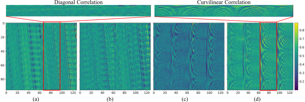
To investigate this limitation, we conducted experiments examining how the embeddings generated by LLMs from time series data relate to the resulting predictions (see Section 2). These embeddings represent the LLMs' reinterpretation of the data, and their correlation with prediction outcomes sheds light on the model's ability to capture relevant patterns. As illustrated in Figure 1(a), when only time-domain signals are used as input, the embeddings exhibit diagonal correlations over just a few time steps. This indicates that the predictions are influenced by a small subset of embeddings, revealing the model's inability to capture broader global correlations. Additionally, certain regions display lower weight values, suggesting the presence of redundant information that diminishes the relevance of these embeddings to the predictions. This points to the need for an approach that better captures global patterns while reducing redundancy.
∗Corresponding Author.
While frequency-domain signals have proven effective in capturing global features of time series (e.g., periodicity and regularity) in non-LLM-based TSF models [Zhou et al., 2022; Yi et al., 2024; Liu and Chen, 2024], their role in LLMbased TSF remains underexplored. Motivated by the limitations observed above, we conducted a preliminary study integrating frequency-domain signals into LLM-based TSF models. Our analysis shows that incorporating these signals into both the prompt and sequence inputs yields curvilinear correlations (see Figure 1(d)) spanning longer time steps-enabling the model to consider a broader information range at each prediction step. Furthermore, the global weight distribution becomes more uniform, alleviating the redundancy found in purely time-domain embeddings and providing a stronger global perspective. These findings underscore the benefits of leveraging frequency-domain signals across both prompt and sequence inputs, thereby enhancing the LLM's ability to interpret and forecast time series data more accurately.
Although incorporating frequency-domain signals into both the prompt and sequence data sections significantly enhances a model's ability to capture key patterns and global features, it also introduces several challenges. One fundamental issue is the mismatch between LLMs-operating on discrete tokens-and the continuous nature of both timedomain and frequency-domain signals [Jin et al., 2024; Pan et al., 2024], which complicates their processing and interpretation. Moreover, the pre-trained knowledge and reasoning capabilities of LLMs are not inherently tailored to these intricate signal patterns, posing ongoing difficulties in achieving accurate and generalizable performance across TSF tasks.
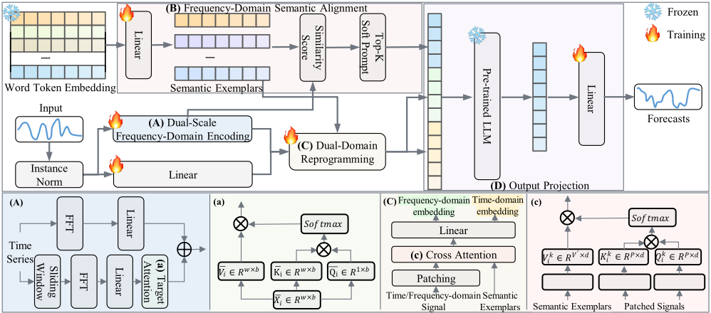
In response to these challenges, we present FreqLLM, a novel framework that seamlessly integrates frequencydomain information into LLMs for TSF, thus capturing global time series patterns to complement local pattern modeling in the time domain. FreqLLM is composed of three key modules: (i) Dual-Scale Frequency-Domain Encoding: Thismodule encodes both global and local frequency-domain signals, ensuring that embeddings capture comprehensive information. By focusing on broader frequency trends as well as local patterns near prediction time points, it preserves both extended and immediate context. (ii) To enhance the LLM's contextual understanding of frequency-domain information, we develop prompts that align with the model's pre-trained semantic knowledge. By integrating task-specific TSF semantics with pre-trained word embeddings, we generate Semantic Exemplars that serve as prompts. These prompts closely align with the frequency-domain embeddings, helping the model more effectively interpret global and local trends in the data. (iii) This module bridges the gap between timedomain and frequency-domain data by reprogramming these signals into embeddings optimized for the LLM's semantic interpretation. By embedding numerical scales and variations from both domains, the model can reason across global and local scales with greater accuracy. To summarize, our main contributions are as follows:
- Investigating the Role of Frequency-Domain Signals in LLM-based TSF: We show that relying solely on timedomain signals in LLM-based TSF leads to diagonal correlations, capturing limited local patterns. In contrast, incorporating frequency-domain signals produces curvilinear correlations, enabling broader global trend modeling and improving forecasting accuracy.
- Introducing FreqLLM: We propose a novel framework that integrates dual-scale frequency-domain embeddings with pre-trained word embeddings. By reprogramming
both time-domain and frequency-domain signals into optimized representations, FreqLLM significantly enhances the ability to capture global patterns and boosts forecast precision.
- Empirical Validation: Extensive experiments on multiple benchmark datasets demonstrate FreqLLM's superior performance compared to existing methods, underscoring the importance of frequency-domain information in LLM-based TSF.
2 Frequency-Domain Signal Learning Patterns Analysis
We constructed four variant models based on the fundamental LLM-based TSF framework [Zhou et al., 2023] to visualize learned model weights. We incorporated a soft prompt component to explore how different prompt and sequence inputs affect the model [Pan et al., 2024]. As illustrated in Figure 1, we categorize inputs into time-domain and frequency-domain data: the former uses the original sequence, while the latter transforms the input into the frequency-domain and concatenates real and imaginary parts of the spectrum as a substitute. We then train the models and visualize their final linear layer weights, which most directly reflect the relationship between the LLM's embeddings and its predictions.
Our experiments use the Traffic dataset with an input window of 512 and a prediction length of 96, maintaining all other settings from the original paper. In Figure 1, the vertical axis represents the 96 forecast values, and the horizontal axis denotes the embedding dimensions output by the LLM (we display the first 128 dimensions for illustration; subsequent values follow a similar pattern).
Figure 1(a): Both the prompt and sequence sections rely on time-domain data. The learned weights form notable diagonal correlations, suggesting the model primarily captures relationships between adjacent time points. However, these diagonals are uneven, with some regions displaying lower weight values-indicative of redundant information that weakens the embeddings' connection to the predictions.
Figure 1(b): The prompt uses frequency-domain data, while the sequence still uses time-domain data. Diagonal correlations persist but are more uniform, with fewer low-weight regions. This points to a stronger link between the embeddings and the prediction results.
Figure 1(c): The prompt relies on time-domain data, whereas the sequence adopts frequency-domain data. The diagonal correlations evolve into arc-like patterns, connecting a broader range of time points and offering a stronger global perspective. However, some areas of lower weight remain, indicating that while global correlations improve, the model's perspective is not yet fully optimized.
Figure 1(d): Both the prompt and sequence sections use frequency-domain data. The weight patterns display comprehensive arc-like correlations spanning nearly the entire embedding space, indicating that the model gains its most extensive global view under this configuration.
3 Methodology
As shown in Figure 2, FreqLLM comprises three key components. The Dual-Scale Frequency Encoding module captures both global and local frequency-domain information, ensuring comprehensive embeddings. The Semantic Alignment module generates task-specific Semantic Exemplars as soft prompts, enhancing the LLM's understanding of frequencydomain patterns. Finally, the Integration and Alignment module bridges time- and frequency-domain representations, optimizing them for the LLM's semantic space to improve prediction accuracy. In this paper, we use GPT-2 [Radford et al., 2019] as the backbone model and don't fine-tune the model during either training or inference, following similar practices in prior works [Pan et al., 2024; Liu et al., 2024a].
3.1 ProblemFormulation
We first formalize the TSF task based on LLMs: Given a time series X ∈ RN×T , representing N different univariate variables over T time steps, the goal is to input X and its frequency-domain representation Xf into an LLMbased predictive module LLM(·), which processes both timedomain and frequency-domain information. The LLM generates forecasts for the subsequent L time steps, denoted as ˆ Y = LLM(X,Xf), ˆ Y ∈ RN×L. The objective is to minimize the Mean Squared Error (MSE) between the predicted values ˆ Y and the actual values Y , defined as:
3.2 Input Embedding
For multivariate time series, different variables exhibit distinct patterns. Directly mixing them and projecting into a unified space makes learning challenging. Thus, we divide the multivariate time series into N univariate time series and process each of them separately [Nie et al., 2023]. Each sequence Xi ∈ R1×T is independently normalized using Reversible Instance Normalization (RevIN) to ensure zero mean and unit variance, reducing distribution shift [Kim et al., 2021]. For ease of reading, we will use X to represent Xi for each channel in the following text.
3.3 Dual-Scale Frequency-Domain Encoding
In the process of transforming time-domain signals into frequency-domain embeddings, we utilize both global and local frequency-domain signals to guide the encoding process. In TSF, both the global and short-term signals of a sequence are important: global signals reflect long-term trends or periodic information, while short-term signals capture changes over a shorter period. In our model, we encode both global and local frequency-domain signals, ensuring that the frequency information of the entire time window is extracted while enhancing the understanding of recent changes. The detailed process of this part is illustrated in Figure 2(A).
For global signals, we first apply a Fast Fourier Transform (FFT) to the normalized time series X, obtaining the global frequency-domain signals. However, not all frequencydomain information is useful. Noise in time series data leads to long-tailed frequency distributions in the frequency domain [Wang et al., 2024]. Therefore, after performing the FFT, we apply a linear layer to filter out the useful frequency information. The specific formula is as follows:
where fglobal is the global frequency-domain embedding.
For local signals, we adopt a target attention mechanism to extract them. The attention mechanism [Vaswani et al., 2017] can dynamically handle relationships between different time steps and focus on important time steps, making it widely applied in time series forecasting. Target attention, developed from the basic attention mechanism, is widely used in recommendation systems [Chen et al., 2021]. Specifically, target attention emphasizes the relationship between specific time steps and global signals, allowing it to highlight the relationship between local and global signals. In detail, as shown in Figure 2(a), we divide X using a sliding window and apply FFT and frequency extraction on each small window, yielding ¯X. The most recent window is used as the query matrices ¯Q, containing the local information closest to the prediction point. The remaining windows serve as the key matrices ¯K and value matrices ¯ V of the target attention. Finally, a linear layer is employed to help the model extract the most important and useful parts of the local frequency information during training. The specific formula is as follows:
where flocal is the global frequency-domain embedding.
After obtaining the global and local frequency-domain signals, we concatenate the two to generate the final frequencydomain embedding ffre:
3.4 Frequency-Domain Semantic Alignment
The prompt is an effective method for activating LLMs to perform better on specific domain tasks [Yin et al., 2023]. In time series analysis, most works focus on template-based and fixed prompts [Xue and Salim, 2023; Jin et al., 2024], but this overlooks the lack of human semantics in time series data, making it difficult for the LLM to understand both the sequence and the prompt. Some works use soft prompts, generating task-specific, trainable vectors to guide the LLM [Sun et al., 2024; Pan et al., 2024]. However, these methods focus on time-domain signals, neglecting the instability and local fluctuations in time series data. In contrast, our model generates soft prompts from frequency-domain signals to provide a broader perspective and address these challenges.
Specifically, we compress the pre-trained word embeddings from the backbone E ∈ RV×D , and employ a simple linear probe to generate semantic exemplars E′ ∈ RV ′×D , where V ′ ≪ V . This linear probing aims to filter out word vectors irrelevant to TSF tasks and consolidate relevant ones, thereby reducing computational costs and concentrating semantic information. Next, we calculate the similarity score between the frequency-domain embedding ffre and the semantic exemplars E′ , which serves as the basis for selecting the exemplars as prompts. The formula is as follows:
where e′n ∈ E′ . Based on the similarity scores, we select K semantic exemplars E′k that best represent the frequency domain information. These K exemplars are concatenated to form the final prompt:
3.5 Dual-Domain Reprogramming
In this section, we reprogram time-domain and frequencydomain signals into semantic exemplars, aligning sequence patterns with natural language structures. This alignment enables the LLM to deliver accurate and generalizable performance across different domains in time series forecasting [Jin et al., 2024]. As discussed earlier, incorporating frequency-domain signals is crucial for capturing both global and local sequence dynamics, while time-domain signals help the LLM understand the sequence's range and average levels. However, since LLMs process discrete tokens and timedomain/frequency-domain signals are continuous, this creates a mismatch in data representation. To address this, we apply a multi-head cross attention mechanism, reprogramming the signals into a format that the LLM can more easily interpret through semantic exemplars.
We divide the signals into overlapping or non-overlapping patches [Nie et al., 2023], each with a length Lp. Therefore, the total number of input patches is P = ⌊ (T-Lp) S ⌋ + 2, where S represents the horizontal sliding stride. A simple linear layer is then used to map the dimensions to dm. After applying the same operation to both signals, we obtain the patched time-domain and frequency-domain signals, denoted as Xtime and Xfre, respectively.
Next, we reprogram the signals into the semantic exemplar space. In constructing the exemplar-aligned prompts, we have obtained a series of semantic exemplars E′ , which retain time series-related word embeddings while reducing semantic dispersion. We use these exemplars to reformat the signals into a more LLM-friendly structure. To achieve this, we apply a multi-head cross-attention mechanism (Figure 2(c)). Specifically, for each head m = {1, · · · ,M}, we define the query matrix ˆ Qm, key matrix ˆ Km, and value matrix ˆ Vm as follows:
where W Q m ∈ Rdm×d , W K m ,W Vm ∈ RD×d , Xsingal is Xtime or Xfre, D is the hidden dimension of the backbone model, and d = ⌊ dm m ⌋.
The reprogramming operation of the signals is defined as:
By aggregating each Zm ∈ RP×d across all heads, we obtain Z ∈ RP×dm . A linear projection is then performed to align the hidden dimensions with the backbone model. After applying the aforementioned operations to both the timedomain and frequency-domain signals, we obtain the timedomain embedding Stime and frequency-domain embedding Sfre, Stime, Sfre ∈ RP×D .
3.6 Output Projection and Optimization Objective
Finally, we integrate the prompt, frequency-domain embedding, and time-domain embedding, which are then fed into the frozen LLM to obtain the output. The output is passed through a linear projection layer to yield the final prediction ˆ Y :
During each training iteration, our optimization objective L is:
where λ ≥ 0 is a trade-off hyperparameter. The first term in the objective function represents the prediction loss of the model, focusing on improving model performance. The second term is the similarity score loss, which averages the similarity scores between the K semantic exemplars selected by the semantic exemplar-aligned prompts and the frequencydomain embedding. The goal of this term is to ensure that the selected semantic exemplars and the frequency-domain embedding are aligned, thus optimizing the soft prompt.
4 Experiments
In this section, we validate the effectiveness and adaptability of the proposed FreqLLM method through experiments. Specifically, we address the following research questions (RQs): 1) Can the proposed FreqLLM model be effectively generalized to long-period time series forecasting scenarios? 2) Can the proposed FreqLLM model be effectively generalized to short-period time series forecasting scenarios? 3) Can the proposed FreqLLM model generate accurate forecasting with limited training data? 4) Are the main modules of the model essential for the FreqLLM method? 5) How do the model's hyperparameters affect its overall forecasting performance? We used a unified pipeline following the experimental configurations of all baselines [Wu et al., 2023].
4.1 Experimental Setup
Datasets: For the long-term forecasting experiments, we test using a variety of datasets, including the Electricity Transformer Temperature (ETT) dataset [Zhou et al., 2021], as well as weather and traffic datasets [Wu et al., 2023], which are widely used for evaluating the long-term forecasting performance of time series models. For short-term experiments, we primarily utilize the M4 benchmark dataset [Makridakis et al., 2018], which consists of time series data from annual, quarterly, monthly, and other categories, featuring large scale, wide coverage, and high-quality data.
Baselines: The baselines include a set of Transformer based methods: PatchTST [Nie et al., 2023], FEDformer [Zhou et al., 2022], Autoformer [Wu et al., 2021], and Informer [Zhou et al., 2021]. We also compared against a set of non-Transformer-based methods: DLinear [Zeng et al., 2023] and TimesNet [Wu et al., 2023]. Lastly, three LLM-based methods, GPT4TS [Zhou et al., 2023], S2 IP-LLM [Pan et al., 2024], and Time-LLM [Jin et al., 2024], were included.
Implementation Details: Our method is trained with MSE loss, using the Adam [Kinga et al., 2015] optimizer with an initial learning rate of 10-2 . We maintain the backbone model at 32 layers. We set the patch dimension dm to 16, the number of heads M to 8, the semantic exemplars size V ′ to 1000, the loss weight λ to 0.08, the sliding window size to 8, and the prompt length K to 8.
4.2 Long-TermForecasting (RQ1)
Setups: For long-term forecasting, we evaluate the effectiveness of FreqLLM on the ETTh1, ETTh2, ETTm1, ETTm2, Weather, and Traffic datasets, which are widely used benchmark datasets for long-term forecasting tasks. The input time series length is set to 512, and we assess performance over four different forecasting horizons: 96, 192, 336, 720. Evaluation metrics include Mean Squared Error (MSE) and Mean Absolute Error (MAE).
Results: Our results are briefly summarized in Table 1. FreqLLM outperforms all baselines in most cases. Compared to models related to LLMs, FreqLLM improves average performance by 2.21% over models that do not fine-tune the backbone, such as Time-LLM, and by 3.88% over models that fine-tune the backbone, such as GPT4TS. FreqLLM achieves a 3.83% improvement in average performance compared to the state-of-the-art task-specific Transformer model PatchTST. This is because (1) FreqLLM leverages both timedomain and frequency-domain data, allowing the model to retain the numerical scale of the data while improving its ability to capture a global perspective, and (2) the semantics exemplars related to TSF tasks, inductively integrated from the pre-trained word embeddings of the LLM, further enhance the representation of the time series.
4.3 Short-TermForecasting (RQ2)
Setups: We use the M4 benchmark [Makridakis et al., 2018] as our test platform. The M4 benchmark dataset is widely recognized as a comprehensive test platform, featuring datasets from various domains such as finance, economics, demographics, and industry. For this setup, the prediction horizon ranges from 6 to 48. The input length is set to twice the prediction horizon. Evaluation metrics include Symmetric Mean Absolute Percentage Error (SMAPE), Mean Absolute Scaled Error (MASE), and Overall Weighted Average (OWA).
| Methods | FreqLLM | S2 IP-LLM | Time-LLM | GPT4TS | PatchTST | FEDformer | DLinear | TimesNet | Autoformer | Informer | ||||||||||
|---|---|---|---|---|---|---|---|---|---|---|---|---|---|---|---|---|---|---|---|---|
| MSE | MAE | MSE | MAE | MSE | MAE | MSE | MAE | MSE | MAE | MSE | MAE | MSE | MAE | MSE | MAE | MSE | MAE | MSE | MAE | |
| ETTh1 | 0.404 | 0.420 | 0.417 | 0.426 | 0.412 | 0.424 | 0.417 | 0.433 | 0.442 | 0.465 | 0.442 | 0.473 | 0.420 | 0.435 | 0.452 | 0.450 | 0.504 | 0.497 | 1.039 | 0.803 |
| ETTh2 | 0.344 | 0.384 | 0.353 | 0.387 | 0.353 | 0.394 | 0.360 | 0.396 | 0.376 | 0.416 | 0.433 | 0.441 | 0.502 | 0.479 | 0.398 | 0.439 | 0.436 | 0.446 | 4.273 | 1.714 |
| ETTm1 | 0.353 | 0.382 | 0.359 | 0.390 | 0.353 | 0.384 | 0.355 | 0.380 | 0.356 | 0.392 | 0.451 | 0.450 | 0.355 | 0.386 | 0.412 | 0.417 | 0.592 | 0.526 | 0.965 | 0.734 |
| ETTm2 | 0.248 | 0.312 | 0.256 | 0.320 | 0.253 | 0.315 | 0.266 | 0.327 | 0.271 | 0.328 | 0.302 | 0.344 | 0.275 | 0.350 | 0.280 | 0.344 | 0.334 | 0.367 | 1.411 | 0.817 |
| Weather | 0.220 | 0.252 | 0.235 | 0.262 | 0.230 | 0.260 | 0.240 | 0.268 | 0.221 | 0.258 | 0.308 | 0.363 | 0.245 | 0.302 | 0.254 | 0.285 | 0.337 | 0.397 | 0.640 | 0.551 |
| Traffic | 0.388 | 0.290 | 0.403 | 0.305 | 0.402 | 0.302 | 0.417 | 0.296 | 0.392 | 0.277 | 0.614 | 0.378 | 0.431 | 0.293 | 0.623 | 0.327 | 0.617 | 0.377 | 0.757 | 0.416 |
| Methods | FreqLLM | S2 IP-LLM | Time-LLM | GPT4TS | PatchTST | FEDformer | DLinear | TimesNet | Autoformer | Informer |
|---|---|---|---|---|---|---|---|---|---|---|
| SMAPE | 11.911 | 12.491 | 12.460 | 12.683 | 12.061 | 13.158 | 13.802 | 12.894 | 12.925 | 14.090 |
| Avg. MASE | 1.618 | 1.652 | 1.646 | 1.816 | 1.630 | 1.782 | 2.051 | 1.795 | 1.789 | 2.742 |
| OWA | 0.876 | 0.884 | 0.906 | 0.986 | 0.892 | 1.006 | 1.053 | 0.960 | 1.024 | 1.279 |
| Percentage | 5% | 10% | ||||||||||||||
|---|---|---|---|---|---|---|---|---|---|---|---|---|---|---|---|---|
| Methods | FreqLLM | S2 IP-LLM | GPT4TS | iTransformer | FreqLLM | S2 IP-LLM | GPT4TS | iTransformer | ||||||||
| MSE | MAE | MSE | MAE | MSE | MAE | MSE | MAE | MSE | MAE | MSE | MAE | MSE | MAE | MSE | MAE | |
| ETTh1 | 0.635 | 0.544 | 0.650 | 0.550 | 0.681 | 0.560 | 1.070 | 0.710 | 0.582 | 0.519 | 0.593 | 0.529 | 0.590 | 0.525 | 0.910 | 0.860 |
| ETTh2 | 0.387 | 0.420 | 0.380 | 0.413 | 0.400 | 0.433 | 0.488 | 0.475 | 0.406 | 0.427 | 0.419 | 0.439 | 0.397 | 0.421 | 0.489 | 0.483 |
| ETTm1 | 0.419 | 0.432 | 0.455 | 0.446 | 0.472 | 0.450 | 0.784 | 0.596 | 0.422 | 0.437 | 0.455 | 0.435 | 0.464 | 0.441 | 0.728 | 0.565 |
| ETTm2 | 0.287 | 0.331 | 0.296 | 0.342 | 0.308 | 0.346 | 0.356 | 0.388 | 0.279 | 0.325 | 0.284 | 0.332 | 0.293 | 0.335 | 0.336 | 0.373 |
| Traffic | 0.414 | 0.280 | 0.420 | 0.299 | 0.434 | 0.305 | 0.450 | 0.324 | 0.434 | 0.311 | 0.427 | 0.307 | 0.440 | 0.310 | 0.495 | 0.361 |
| Weather | 0.277 | 0.316 | 0.260 | 0.297 | 0.263 | 0.301 | 0.309 | 0.339 | 0.233 | 0.265 | 0.233 | 0.272 | 0.238 | 0.275 | 0.308 | 0.338 |
Results: Table 2 summarizes the short-term forecasting results. We observe that FreqLLM consistently outperforms all baselines, showing improvements of 3.15% and 9.39% over Time-LLM and GPT4TS, respectively. FreqLLM remains competitive even when compared with the SOTA model, PatchTST. This could be attributed to the focus on utilizing local frequency-domain signals closest to the prediction time period, which helps identify the most relevant influencing information for the prediction points, mitigating the issue of missing correlations caused by short sequence lengths.
4.4 Few-Shot Learning (RQ3)
Setups: We follow the experimental setup in [Zhou et al., 2023] to evaluate the performance under the few-shot prediction setting, which allows us to examine whether the model can generate accurate predictions with limited data. In these experiments, we use the top 5% and 10% of the training data.
Results: We summarize the few-shot learning experiment results in Table 3. We observed that LLM-based methods, such as S2 IP-LLM and GPT4TS, significantly outperform other baseline methods. This is because other baseline methods are trained from scratch and have limited training data in this case. On the other hand, FreqLLM leverages frequency domain information to help the model learn more domainrelevant knowledge, thereby improving its performance in few-shot learning.
4.5 Ablation Studies (RQ4)
Setups: We conducted an ablation study on the ETTh1 and ETTh2 datasets to verify the necessity of the three key components of FreqLLM. To verify the effectiveness of the LLM in our model, we follow the experimental setup in [Tan et al., 2024] which the LLM is removed, while retaining the remaining components of the model, and compare the performance. We created four FreqLLM variants:
- FreqLLM v1: Replaces the Dual-Scale FrequencyDomain Encoding with an FFT.
- FreqLLM v2: Replaces the Frequency-Domain Semantic Alignment module with a linear layer.
- FreqLLM v3: Replaces the Dual-Domain Reprogramming module with two linear layers.
- FreqLLMv4: Removes the LLM components, retaining only the remaining structure.
Results: The experimental results are shown in Table 4. It can be observed that these three components are effective for FreqLLM in the vast majority of cases. Among them, Dual-Domain Reprogramming contributed the most improvement to the model, with an average performance gain of 4.97%. Dual-Scale Frequency-Domain Encoding had a slightly smaller impact, with an average improvement of 1.94%, while Frequency-Domain Semantic Alignment fell between the two, offering an average performance boost of 3.24%. Notably, removing the LLM results in a 1.85% performance decline, underscoring its critical role in the model.
| Methods | ETTh1-96 | ETTh1-192 | ETTh1-336 | ETTh1-720 | ETTh2-96 | ETTh2-192 | ETTh2-336 | ETTh2-720 | ||||||||
|---|---|---|---|---|---|---|---|---|---|---|---|---|---|---|---|---|
| MSE | MAE | MSE | MAE | MSE | MAE | MSE | MAE | MSE | MAE | MSE | MAE | MSE | MAE | MSE | MAE | |
| FreqLLM v1 | 0.378 | 0.392 | 0.407 | 0.419 | 0.421 | 0.432 | 0.454 | 0.466 | 0.287 | 0.345 | 0.337 | 0.371 | 0.366 | 0.406 | 0.401 | 0.418 |
| FreqLLM v2 | 0.377 | 0.409 | 0.427 | 0.428 | 0.440 | 0.446 | 0.439 | 0.448 | 0.294 | 0.358 | 0.355 | 0.385 | 0.358 | 0.392 | 0.418 | 0.447 |
| FreqLLM v3 | 0.381 | 0.407 | 0.431 | 0.431 | 0.437 | 0.444 | 0.452 | 0.466 | 0.301 | 0.364 | 0.362 | 0.399 | 0.373 | 0.419 | 0.414 | 0.453 |
| FreqLLM v4 | 0.370 | 0.395 | 0.414 | 0.421 | 0.419 | 0.424 | 0.440 | 0.462 | 0.299 | 0.354 | 0.353 | 0.381 | 0.355 | 0.400 | 0.405 | 0.432 |
| FreqLLM | 0.367 | 0.390 | 0.406 | 0.414 | 0.411 | 0.426 | 0.434 | 0.451 | 0.285 | 0.340 | 0.344 | 0.378 | 0.350 | 0.392 | 0.396 | 0.427 |

4.6 Parameter Sensitivity (RQ5)
Setups: We conducted a Parameter Sensitivity experiment on the ETTh1 and ETTh2 datasets to assess FreqLLM's adaptability to different hyperparameters. The results, shown in Figures 3, demonstrate how FreqLLM performs in various settings for semantic exemplar size, loss weight, prompt length, and GPT-2 layer count.
Results: The experimental results in Figure 3 show that as the size of semantic exemplars V ′ increases, MSE on ETTh1 and ETTh2 remains stable with minor fluctuations, decreasing until a certain point and then rising. This suggests that a small V ′ leads to limited information, while a large V ′ introduces irrelevant data. For the loss weight λ, a moderate value improves prediction, while a larger λ reduces performance. Similarly, increasing the prompt length (K) improves accuracy up to a point, but excessively long prompts reduce focus on the most relevant information, decreasing accuracy. With the increase in GPT-2 layers, performance continuously improves, as deeper architectures capture more complex time series patterns. These results demonstrate FreqLLM's adaptability to various hyperparameters.
5 RelatedWork
5.1 Time Series Forecasting
Given the importance of TSF, various models have been developed. Transformer-based models have been widely explored and refined for TSF [Zhou et al., 2021; Wu et al., 2021; Lin et al., 2024]. Recent research has focused on optimizing Transformers' capabilities in handling time series data, such as PatchTST [Nie et al., 2023], which aggregates time steps into patches, and iTransformer [Liu et al., 2024b], which reallocates dimensions to enhance multivariate correlations, has significantly boosted model performance. Meanwhile, traditional linear and TCN-based models, with specific modifications, have demonstrated performance comparable to Transformer-based models while circumventing the slower training speeds associated with Transformers [Zeng et al., 2023; Das et al., 2023; Wu et al., 2023]. These methods perform well on specific tasks but require task-specific training and lack cross-domain generalization.
5.2 Large Language Models for Time Series Forecasting
With the rise of large language models (LLMs), researchers have developed TSF models that leverage LLMs' pattern recognition capabilities [Cui et al., 2024; He et al., 2022b; Ghosal et al., 2023]. Some methods convert time series data into textual formats for LLM input, such as LLMTIME [Gruver et al., 2024] and PromptCast [Xue and Salim, 2023], while others align time series with LLMs' pre-trained semantic space using embeddings and mapping layers, as seen in TEST [Sun et al., 2024], Time-LLM [Jin et al., 2024], and S2 IP-LLM [Pan et al., 2024]. Unlike these approaches, FreqLLM incorporates frequency-domain information to capture underlying periodicity and fluctuations, addressing challenges from instability and local variations in time series data.
6 Conclusion
We propose FreqLLM, a model that incorporates frequencydomain signals to enhance LLMs' understanding of time series data for forecasting. The model captures both global and local patterns from the frequency domain and aligns these signals with the LLM's pre-trained knowledge, improving its contextual understanding. Experiments on benchmark datasets validate FreqLLM's effectiveness. Future work should focus on improving the integration of time and frequency-domain information and exploring multimodal pre-training for greater adaptability in forecasting tasks.
Acknowledgments
Min Gao is supported by the National Natural Science Foundation of China (No. 62176028); Feng Jiang is supported by the Science and Technology Research Program of Chongqing Municipal Education Commission (No. KJZDK202304401); and Guansong Pang is supported in part by A*STAR MTC YIRG Grant (No. M24N8c0103), the Ministry of Education, Singapore under Tier-1 Academic Research Fund (No. 24-SIS-SMU-008), and the Lee Kong Chian Fellowship.
@inproceedings{ijcai2025p377,
  title     = {FreqLLM: Frequency-Aware Large Language Models for Time Series Forecasting},
  author    = {Wang, Shunnan and Gao, Min and Wang, Zongwei and Bai, Yibing and Jiang, Feng and Pang, Guansong},
  booktitle = {Proceedings of the Thirty-Fourth International Joint Conference on
               Artificial Intelligence, {IJCAI-25}},
  publisher = {International Joint Conferences on Artificial Intelligence Organization},
  editor    = {James Kwok},
  pages     = {3389--3397},
  year      = {2025},
  month     = {8},
  note      = {Main Track},
  doi       = {10.24963/ijcai.2025/377},
  url       = {https://doi.org/10.24963/ijcai.2025/377},
}
TY - CPAPER TI - FreqLLM: Frequency-Aware Large Language Models for Time Series Forecasting AU - Wang, Shunnan AU - Gao, Min AU - Wang, Zongwei AU - Bai, Yibing AU - Jiang, Feng AU - Pang, Guansong T2 - Proceedings of the Thirty-Fourth International Joint Conference on Artificial Intelligence, IJCAI-25 PB - International Joint Conferences on Artificial Intelligence Organization PY - 2025 SP - 3389 EP - 3397 DO - 10.24963/ijcai.2025/377 UR - https://doi.org/10.24963/ijcai.2025/377 ER -Copied
Machine-readable versions of this paper, for tools and AI agents:





