
Explainable Graph Representation Learning via Graph Pattern Analysis
Proceedings of the Thirty-Fourth International Joint Conference on Artificial Intelligence. Main Track. Pages 3426-3434.
https://doi.org/10.24963/ijcai.2025/381
Keywords
- Machine Learning: ML: Explainable/Interpretable machine learning
- Machine Learning: ML: Sequence and graph learning
- Data Mining: DM: Mining graphs
Abstract
Explainable artificial intelligence (XAI) is an important area in the AI community, and interpretability is crucial for building robust and trustworthy AI models. While previous work has explored model-level and instance-level explainable graph learning, there has been limited investigation into explainable graph representation learning. In this paper, we focus on representation-level explainable graph learning and ask a fundamental question: What specific information about a graph is captured in graph representations? Our approach is inspired by graph kernels, which evaluate graph similarities by counting substructures within specific graph patterns. Although the pattern counting vector can serve as an explainable representation, it has limitations such as ignoring node features and being high-dimensional. To address these limitations, we introduce a framework (PXGL-GNN) for learning and explaining graph representations through graph pattern analysis. We start by sampling graph substructures of various patterns. Then, we learn the representations of these patterns and combine them using a weighted sum, where the weights indicate the importance of each graph pattern's contribution. We also provide theoretical analyses of our methods, including robustness and generalization. In our experiments, we show how to learn and explain graph representations for real-world data using pattern analysis. Additionally, we compare our method against multiple baselines in both supervised and unsupervised learning tasks to demonstrate its effectiveness.
- [Adadi and Berrada, 2018] Amina Adadi and Mohammed Berrada. Peeking inside the black-box: a survey on explainable artificial intelligence (xai). IEEE access, 6:52138-52160, 2018.
- [Alon et al., 2008] Noga Alon, Phuong Dao, Iman Hajira- souliha, Fereydoun Hormozdiari, and S Cenk Sahinalp. Biomolecular network motif counting and discovery by color coding. Bioinformatics, 24(13):i241-i249, 2008.
- [Angelov et al., 2021] Plamen P Angelov, Eduardo A Soares, Richard Jiang, Nicholas I Arnold, and Peter M Atkinson. Explainable artificial intelligence: an analyti- cal review. Wiley Interdisciplinary Reviews: Data Mining and Knowledge Discovery, 11(5):e1424, 2021.
- [Azzolin et al., 2022] Steve Azzolin, Antonio Longa, Pietro Barbiero, Pietro Liò, and Andrea Passerini. Global ex- plainability of gnns via logic combination of learned con- cepts. arXiv preprint arXiv:2210.07147, 2022.
- [Borgwardt et al., 2005] Karsten M Borgwardt, Cheng Soon Ong, Stefan Schönauer, SVN Vishwanathan, Alex J Smola, and Hans-Peter Kriegel. Protein function predic- tion via graph kernels. Bioinformatics, 21(suppl 1):i47- i56, 2005.
- [Bousquet and Elisseeff, 2002] Olivier Bousquet and André Elisseeff. Stability and generalization. The Journal of Ma- chine Learning Research, 2:499-526, 2002.
- [Da San Martino et al., 2012] Giovanni Da San Martino, Ni- colo Navarin, and Alessandro Sperduti. A tree-based ker- nel for graphs. In Proceedings of the 2012 SIAM Interna- tional Conference on Data Mining, pages 975-986. SIAM, 2012.
- [Feldman and Vondrak, 2019] Vitaly Feldman and Jan Von- drak. High probability generalization bounds for uni- formly stable algorithms with nearly optimal rate. In Con- ference on Learning Theory, pages 1270-1279. PMLR, 2019.
- [Fox et al., 2020] Jacob Fox, Tim Roughgarden, C Se- shadhri, Fan Wei, and Nicole Wein. Finding cliques in social networks: A new distribution-free model. SIAM journal on computing, 49(2):448-464, 2020.
- [Gärtner et al., 2003] Thomas Gärtner, Peter Flach, and Ste- fan Wrobel. On graph kernels: Hardness results and effi- cient alternatives. In Learning theory and kernel machines, pages 129-143. Springer, 2003.
- [Girvan and Newman, 2002] Michelle Girvan and Mark EJ Newman. Community structure in social and biological networks. Proceedings of the national academy of sci- ences, 99(12):7821-7826, 2002.
- [Hamilton et al., 2017] Will Hamilton, Zhitao Ying, and Jure Leskovec. Inductive representation learning on large graphs. Advances in neural information processing sys- tems, 30, 2017.
- [Hassija et al., 2024] Vikas Hassija, Vinay Chamola, Atmesh Mahapatra, Abhinandan Singal, Divyansh Goel, Kaizhu Huang, Simone Scardapane, Indro Spinelli, Mufti Mahmud, and Amir Hussain. Interpreting black-box models: a review on explainable artificial intelligence. Cognitive Computation, 16(1):45-74, 2024.
- [Huang and Villar, 2021] Ningyuan Teresa Huang and Soledad Villar. A short tutorial on the weisfeiler-lehman test and its variants. In ICASSP 2021-2021 IEEE Inter- national Conference on Acoustics, Speech and Signal Processing (ICASSP), pages 8533-8537. IEEE, 2021.
- [Huang et al., 2023] Zexi Huang, Mert Kosan, Sourav Me- dya, Sayan Ranu, and Ambuj Singh. Global counterfactual explainer for graph neural networks. In Proceedings of the Sixteenth ACM International Conference on Web Search and Data Mining, pages 141-149, 2023.
- [Jiang et al., 2010] Chuntao Jiang, Frans Coenen, and Michele Zito. Finding frequent subgraphs in longitudi- nal social network data using a weighted graph mining approach. In Advanced Data Mining and Applications: 6th International Conference, ADMA 2010, Chongqing, China, November 19-21, 2010, Proceedings, Part I 6, pages 405-416. Springer, 2010.
- [Kipf and Welling, 2016] Thomas N Kipf and Max Welling. Semi-supervised classification with graph convolutional networks. arXiv preprint arXiv:1609.02907, 2016.
- [Kosan et al., 2023] Mert Kosan, Samidha Verma, Burouj Armgaan, Khushbu Pahwa, Ambuj Singh, Sourav Medya, and Sayan Ranu. Gnnx-bench: Unravelling the utility of perturbation-based gnn explainers through in-depth bench- marking. arXiv preprint arXiv:2310.01794, 2023.
- [Kriege and Mutzel, 2012] Nils Kriege and Petra Mutzel. Subgraph matching kernels for attributed graphs. arXiv preprint arXiv:1206.6483, 2012.
- [Kriege et al., 2020] Nils M Kriege, Fredrik D Johansson, and Christopher Morris. A survey on graph kernels. Ap- plied Network Science, 5:1-42, 2020.
- [Luo et al., 2020] Dongsheng Luo, Wei Cheng, Dongkuan Xu, Wenchao Yu, Bo Zong, Haifeng Chen, and Xiang Zhang. Parameterized explainer for graph neural net- work. Advances in neural information processing systems, 33:19620-19631, 2020.
- [Luo et al., 2023] Xiao Luo, Wei Ju, Yiyang Gu, Zhengyang Mao, Luchen Liu, Yuhui Yuan, and Ming Zhang. Self- supervised graph-level representation learning with adver- sarial contrastive learning. ACM Transactions on Knowl- edge Discovery from Data, 2023.
- [Morgan, 1965] Harry L Morgan. The generation of a unique machine description for chemical structures-a technique developed at chemical abstracts service. Journal of chem- ical documentation, 5(2):107-113, 1965.
- [Morris et al., 2020] Christopher Morris, Nils M. Kriege, Franka Bause, Kristian Kersting, Petra Mutzel, and Mar- ion Neumann. Tudataset: A collection of benchmark datasets for learning with graphs. In ICML 2020 Workshop on Graph Representation Learning and Beyond (GRL+ 2020), 2020.
- [O'Bray et al., 2021] Leslie O'Bray, Max Horn, Bastian Rieck, and Karsten Borgwardt. Evaluation metrics for graph generative models: Problems, pitfalls, and practical solutions. arXiv preprint arXiv:2106.01098, 2021.
- [Oord et al., 2018] Aaron van den Oord, Yazhe Li, and Oriol Vinyals. Representation learning with contrastive predic- tive coding. arXiv preprint arXiv:1807.03748, 2018.
- [O'Boyle and Sayle, 2016] Noel M O'Boyle and Roger A Sayle. Comparing structural fingerprints using a literature- based similarity benchmark. Journal of cheminformatics, 8:1-14, 2016.
- [Pržulj, 2007] Nataša Pržulj. Biological network compar- ison using graphlet degree distribution. Bioinformatics, 23:e177-e183, 2007.
- [Rahman et al., 2009] Syed Asad Rahman, Matthew Bash- ton, Gemma L Holliday, Rainer Schrader, and Janet M Thornton. Small molecule subgraph detector (smsd) toolkit. Journal of cheminformatics, 1:1-13, 2009.
- [Smola and Vishwanathan, 2002] Alex Smola and SVN Vishwanathan. Fast kernels for string and tree matching. Advances in neural information processing systems, 15, 2002.
- [Sun and Fan, 2024] Yan Sun and Jicong Fan. Mmd graph kernel: Effective metric learning for graphs via maximum mean discrepancy. In ICLR, 2024.
- [Sun et al., 2019] Fan-Yun Sun, Jordan Hoffmann, Vikas Verma, and Jian Tang. Infograph: Unsupervised and semi-supervised graph-level representation learning via mutual information maximization. arXiv preprint arXiv:1908.01000, 2019.
- [Sun et al., 2023] Ziheng Sun, Chris Ding, and Jicong Fan. Lovász principle for unsupervised graph representation learning. In Advances in Neural Information Processing Systems, volume 36, pages 58290-58311.
- [Tan et al., 2023] Qiaoyu Tan, Ninghao Liu, Xiao Huang, Soo-Hyun Choi, Li Li, Rui Chen, and Xia Hu. S2gae: self- supervised graph autoencoders are generalizable learners with graph masking. In Proceedings of the sixteenth ACM international conference on web search and data mining, pages 787-795, 2023.
- [Wang and Fan, 2024] Zixiao Wang and Jicong Fan. Graph classification via reference distribution learning: Theory and practice. In Advances in Neural Information Process- ing Systems, volume 37, pages 137698-137740.
- Curran Associates, Inc., 2024.
- [Wang et al., 2020] Pengyang Wang, Yanjie Fu, Yuanchun Zhou, Kunpeng Liu, Xiaolin Li, and Kien A Hua. Ex- ploiting mutual information for substructure-aware graph representation learning. In IJCAI, pages 3415-3421, 2020. IJCAI
- [Wang et al., 2021] Xin Wang, Shuyi Fan, Kun Kuang, and Wenwu Zhu. Explainable automated graph representation learning with hyperparameter importance. In International Conference on Machine Learning, pages 10727-10737.
- PMLR, 2021.
- [Xie et al., 2016] Junyuan Xie, Ross Girshick, and Ali Farhadi. Unsupervised deep embedding for clustering analysis. In International conference on machine learn- ing, pages 478-487. PMLR, 2016.
- [Xu et al., 2018] Keyulu Xu, Weihua Hu, Jure Leskovec, and Stefanie Jegelka. How powerful are graph neural net- works? arXiv preprint arXiv:1810.00826, 2018.
- [Yan et al., 2011] Yan Yan, Shenggui Zhang, and Fang- Xiang Wu. Applications of graph theory in protein struc- ture identification. Proteome science, 9:1-10, 2011.
- [Ying et al., 2018] Zhitao Ying, Jiaxuan You, Christopher Morris, Xiang Ren, Will Hamilton, and Jure Leskovec. Hierarchical graph representation learning with differen- tiable pooling. Advances in neural information processing systems, 31, 2018.
- [Ying et al., 2019] Zhitao Ying, Dylan Bourgeois, Jiaxuan You, Marinka Zitnik, and Jure Leskovec. Gnnexplainer: Generating explanations for graph neural networks. Ad- vances in neural information processing systems, 32, 2019.
- [You et al., 2020] Yuning You, Tianlong Chen, Yongduo Sui, Ting Chen, Zhangyang Wang, and Yang Shen. Graph con- trastive learning with augmentations. Advances in Neural Information Processing Systems, 33:5812-5823, 2020.
- [Yuan et al., 2020] Hao Yuan, Jiliang Tang, Xia Hu, and Shuiwang Ji. Xgnn: Towards model-level explanations of graph neural networks. In Proceedings of the 26th ACM SIGKDD international conference on knowledge discov- ery & data mining, pages 430-438, 2020.
- [Zeng et al., 2023] Dingyi Zeng, Wanlong Liu, Wenyu Chen, Li Zhou, Malu Zhang, and Hong Qu. Substructure aware graph neural networks. In Proceedings of the AAAI Conference on Artificial Intelligence, volume 37, pages 11129-11137, 2023.
- [Zhang et al., 2018] Muhan Zhang, Zhicheng Cui, Marion Neumann, and Yixin Chen. An end-to-end deep learn- ing architecture for graph classification. In Proceedings of the AAAI conference on artificial intelligence, volume 32, 2018.
- [Zhao et al., 2018] Xiaohan Zhao, Bo Zong, Ziyu Guan, Kai Zhang, and Wei Zhao. Substructure assembling network for graph classification. In Proceedings of the AAAI Con- ference on Artificial Intelligence, volume 32, 2018.
- [Zhao et al., 2024] Zhe Zhao, Pengkun Wang, Haibin Wen, Yudong Zhang, Zhengyang Zhou, and Yang Wang. A twist for graph classification: Optimizing causal informa- tion flow in graph neural networks. In Proceedings of the AAAI Conference on Artificial Intelligence, volume 38, pages 17042-17050, 2024.
References were extracted automatically from the PDF and may contain errors.
Full text extracted automatically from the PDF; figures, tables and equations may differ. The PDF is the version of record.
1 Introduction
The research field of explainable artificial intelligence (XAI) [Adadi and Berrada, 2018; Angelov et al., 2021; Hassija et al., 2024] is gaining significant attention in both AI and science communities. Interpretability is crucial for creating robust and trustworthy AI models, especially in critical domains like transportation, healthcare, law, and finance. Graph learning [Sun et al., 2023; Sun and Fan, 2024; Wang and Fan, 2024] is an important area of AI that particularly focuses on graph-structured data that widely exists in social science, biology, chemistry, etc. Explainable graph learning (XGL) [Kosan et al., 2023] can be generally classified into two categories: model-level methods and instancelevel methods.
∗Corresponding author.
Model-level methods of XGL provide transparency by analyzing the model behavior. Examples include XGNN [Yuan et al., 2020], GLG-Explainer [Azzolin et al., 2022], and GCFExplainer [Huang et al., 2023]. Instance-level methods of XGL offer explanations tailored to specific predictions, focusing on why particular instances are classified in a certain manner. For instance, GNNExplainer [Ying et al., 2019] identifies a compact subgraph structure crucial for a GNN's prediction. PGExplainer [Luo et al., 2020] trains a graph generator to incorporate global information and parameterize the explanation generation process. AutoGR [Wang et al., 2021] introduces an explainable AutoML approach for graph representation learning.
However, these works mainly focus on enhancing the transparency of GNN models or identifying the most important substructures that contribute to predictions. The exploration of representation-level explainable graph learning (XGL) is limited. We propose explainable graph representation learning and ask a fundamental question: What specific information about a graph is captured in graph representations? Formally, if we represent a graph G as a d-dimensional vector g, our goal is to understand what specific information about the graph G is embedded in the representation g. This problem is important and has practical applications. Some graph patterns are highly practical and crucial in various real-world tasks, and we want this information to be captured in representations. For instance, in molecular chemistry, bonds between atoms or functional groups often form cycles (rings), which indicate a molecule's properties and can be used to generate molecular fingerprints [Morgan, 1965; Alon et al., 2008; Rahman et al., 2009; O'Boyle and Sayle, 2016]. Similarly, cliques characterize protein complexes in Protein-Protein Interaction networks and help identify community structures in social networks [Girvan and Newman, 2002; Jiang et al., 2010; Fox et al., 2020].
Although some previous works such as [Kosan et al., 2023] aimed to find the most critical subgraph S by solving optimization problems based on perturbation-based reasoning, either factual or counterfactual, this kind of approach assumes that the most important subgraph S mainly contributes to the representation g, neglecting other aspects of the graph, which doesn't align well with our goal of thoroughly understanding graph representations. Analyzing all subgraphs of a graph G is impractical due to their vast number. To address the challenge, we propose to group the subgraphs into different graph patterns, like paths, trees, cycles, cliques, etc, and then analyze the contribution of each graph pattern to the graph representation g.
Our idea of pattern analysis is inspired by graph kernels, which compare substructures of specific graph patterns to evaluate the similarity between two graphs [Kriege et al., 2020]. For example, random walk kernels [Borgwardt et al., 2005; G¨artner et al., 2003] use path patterns, sub-tree kernels [Da San Martino et al., 2012; Smola and Vishwanathan, 2002] examine tree patterns, and graphlet kernels [Prˇzulj, 2007] focus on graphlet patterns. The graph kernel involves learning a pattern counting representation vector h, which counts the occurrences of substructures of a specific pattern within the graph G. While the pattern counting vector h is an explainable representation, it has some limitations, such as the high dimensionality and ignorance of node features.
There also exist some representation methods based on subgraphs and substructures, such as Subgraph Neural Networks (SubGNN) [Kriege and Mutzel, 2012], Substructure Assembling Network (SAN) [Zhao et al., 2018], Substructure Aware Graph Neural Networks (SAGNN) [Zeng et al., 2023], and Mutual Information (MI) Induced Substructureaware GRL [Wang et al., 2020]. However, these methods mainly focus on increasing expressiveness and do not provide explainability for representation learning.
In this work, we propose a novel framework to learn and explain graph representations via graph pattern analysis. We start by sampling graph substructures of various patterns. Then, we learn the representations of these patterns and combine them adaptively, where the weights indicate the importance of each graph pattern's contribution. We also provide theoretical analyses of our methods, including robustness and generalization. Additionally, we compare our method against multiple baselines in both supervised and unsupervised learning tasks to demonstrate its effectiveness and superiority. Our contributions are summarized as follows:
- Unlike previous model-level and instance-level XGL, we introduce a new issue - representation-level explainable graph learning. This issue focuses on understanding what specific information about a graph is embedded within its representations.
- We propose two strategies to learn and explain graph representations, including a graph ensemble kernel method (PXGL-EGK) and a pattern analysis GNN method (PXGL-GNN). The latter involves using GNNs to learn the representations of each pattern and evaluate its contribution to the ensemble graph representation.
- We provide theoretical analyses of our methods, including robustness and generalization.
2 Notations
In this work, we use x, x, X, and X (or X) to denote scalar, vector, matrix, and set, respectively. We denote [n] = {1, 2, ..., n}. Let G = (V,E) be a graph with n nodes and d-dimensional node features {xv ∈ Rd | v ∈ V }. We denote A ∈ {0, 1}n×n the adjacency matrix and X = [x1, . . . , xn]⊤ ∈ Rn×d the node features matrix. Let G = {G1, . . . ,GN} be a dataset of N graphs belonging C classes, where Gi = (Vi,Ei). For Gi, we denote its number of nodes as ni, the one-hot graph label as yi ∈ {0, 1}C , the graph-level representation as a vector gi ∈ Rd , the adjacency matrix as Ai, and the node feature matrix as Xi. Let S = (VS, ES) be a subgraph of graph G = (V, E) such that VS ⊆ V and ES ⊆ E. The the adjacency matrix of S is denoted as AS ∈ {0, 1}|VS|×|VS| and the node feature matrix of S is sampled from the rows of X, denoted as XS ∈ R|VS|×d .
The graph pattern is defined as a set of all graphs that share certain properties, denoted as P = {P1, P2, . . . , Pi, . . .}, where Pi is the i-th example of this pattern. In this work, the graph patterns are basic graph families such as paths, trees, cycles, cliques, etc. For example:
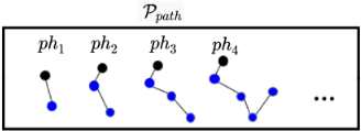
- Ppath = {ph1 , ph2 , . . . , phi , . . .} is a path pattern with phi as a path of length i.
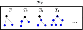
- PT = {T1, T2, . . . , Ti, . . .} is a tree pattern where Ti is the i-th tree.
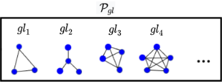
- Pgl = {gl1 , gl2 , . . . , gli , . . .} is a graphlet pattern where gli is the i-th graphlet.
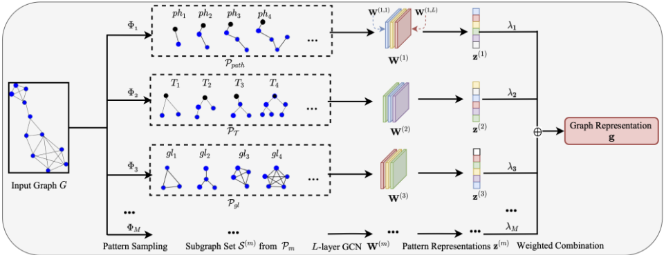
Figure 1 illustrates some intuitive examples of graph patterns. Notably, there are overlaps among different patterns; for instance, the graph T3 ∈ PT and gl2 ∈ Pgl are identical, being both a tree and a graphlet. Overlaps are inevitable due to the predefined nature of these basic graph families in graph theory. We denote a set of M different patterns as {P1,P2, . . . , Pm, . . . , PM}. Given the pattern Pm and the graph Gi, the pattern sampling set is denoted as S (m) i and the pattern representation is denoted as z(m) i ∈ Rd .
3 XGL via Ensemble Graph Kernel
In this section, we learn and explain the pattern counting graph representation via graph kernels.
3.1 Pattern Counting Kernel
A graph kernel K : G × G → R aims to evaluate the similarity between two graphs. Let Gi and Gj be two graphs in the graph dataset G and let H be a high-dimensional vector space. The key to a graph kernel is defining a mapping from the graph space to the high-dimensional vector space as ϕ : G → H, where hi = ϕ(Gi) and hj = ϕ(Gj). Then, the graph kernel can be defined as the inner product of hi and hj, i.e., K(Gi,Gj) := h⊤i hj. The most widely used mapping ϕ is the one counting the occurrences of each example in the pattern P within graph G. The corresponding pattern counting vector is defined as follows:
Definition 3.1 (Pattern Counting Vector). Given a graph G and a pattern P = {P1, P2, . . . , Pi, . . .}, a pattern counting pattern Pm within the dataset G. Instead of the constrained optimization (3), we may consider replacing λm with exp(wm)/ ∑Mm=1 exp(wm) such that the constraints are satisfied inherently, which leads to an unconstrained optimization in terms of w = [w1, . . . ,wM]⊤. In the following context, for convenience, we focus on (3), though all results are applicable to the unconstrained optimization. To obtain the weight parameter λ, we provide the supervised and unsupervised loss functions as follows.
Supervised Contrastive Loss. Following [Oord et al., 2018], given a kernel matrix K ∈ RN×N , we define the supervised InfoNEC loss of K as follows
where I[·] is an indicator function and µ > 0 is a hyperparameter.
Unsupervised KL Divergence. Inspired by [Xie et al., 2016], given a kernel matrix K ∈ RN×N , we define the unsupervised KL divergence loss as follows
where rj are soft cluster frequencies. By minimizing the KL divergence, the model adjusts the parameters λ to more accurately represent the natural clustering property of the dataset.
We use the LSCL or LKL as our loss function, i.e., Lker(λ) = LSCL(K(λ)) or LKL(K(λ)), when the graphs are labeled or unlabeled. Then the weight parameter λ can be obtain by solving
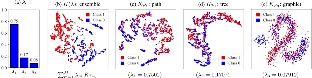
where λ∗ = [λ∗1 , ..., λ∗m, ...λ∗M ]⊤ and λ∗m indicates the importance of kernel KPm as well as pattern Pm. In Figure 2, we can see that the ensemble Kernel performs better than each single kernel and the pattern analysis identifies the importance of each kernel as well as the related graph pattern. We call this method pattern-based XGL with ensemble graph kernel, abbreviated as PXGL-EGK. This method not only yields explainable similarity learning but also provides an approach to selecting graph kernels and their hyperparameters automatically if we consider different kernel types with different hyperparameters.
mapping ϕ : G → H is defined as
where h(i) is the number of occurrences of pattern example Pi as a substructure within graph G. We call h a pattern counting vector of G related to pattern P.
Then the pattern counting kernel KP : G × G → R based on pattern P is defined as:
Definition 3.2 (Pattern Counting Kernel). Given the a pattern counting mapping ϕ(G; P), a pattern counting kernel is defined as
The pattern counting kernel KP is uniquely determined by the pattern P. For example, if P is selected as the path pattern Ppath, we obtain a random walk kernel [Borgwardt et al., 2005; G¨artner et al., 2003]. If P is the tree pattern PT , we get a sub-tree kernel [Da San Martino et al., 2012; Smola and Vishwanathan, 2002]. Similarly, if P is the graphlet pattern Pgl, we derive a graphlet kernel [Prˇzulj, 2007].
3.2 Pattern Analysis Using Graph Kernels
Let {P1, P2, . . . , PM} be a set of M different graph patterns. For instance, P1 represents the path pattern and P2 represents the tree pattern. Then, we can define a set of M different graph kernels as {KP1 ,KP2 , . . . ,KPM }. Since the pattern counting kernel KPm is uniquely determined by the pattern Pm, we can analyse the importance of pattern Pm by evaluating the importance of its pattern counting kernel KPm . To achieve this, we define a learnable ensemble kernel as follows:
Definition 3.3 (Learnable Ensemble Kernel). Let λ = [λ1, λ2, ..., λm, ..., λM]⊤ be a positive weight parameter vector. The ensemble kernel matrix K(λ) ∈ R|G|×|G| is defined as the weighted sum of M different kernels {KP1 ,KP2 , . . . ,KPM }. Given two graphs Gi and Gj in G, the element at the i-th row and j-th column of K(λ) is given by
Here, the weight parameter λm indicates the importance of the kernel KPm as well as the corresponding graph
3.3 Limitations of Pattern Counting Vector
The pattern counting vector h from Definition 3.1 is easy to understand and its importance can be evaluated using the weight parameter λ∗ from (6). However, it cannot directly explain the representation of graph G due to the following limitations:
- Ignoring Node Features: h captures the topology of G but ignores node features X. As shown by previous GNN works, node features are crucial for learning graph representations.
- High Dimensionality: The pattern set P = {P1, P2, . . . , Pi, . . .} can be vast, making h highdimensional and impractical for many tasks.
- Time Complexity: Counting patterns Pi in G is timeconsuming due to the large number of patterns in P. The function ϕ(G; P) needs to be run for each new graph.
- Lacking Implicit Information and Strong Expressiveness: h is fixed and not learnable. GNN [Kipf and Welling, 2016] shows that message passing can learn implicit information and provide better representations, which should be considered if possible.
4 Learning Explainable Graph Representations via GNNs
In this section, we address the limitations pointed out in Section 3.3 by proposing a GNN framework to learn and explain graph representations via pattern analysis. First, we sample graph substructures of various patterns from graph G. Given that overlaps may occur between patterns, we use the WL-test [Huang and Villar, 2021] in each sampling phase to ensure that new samples are unique from existing ones. The pattern sampling set S is defined as follows.
Definition 4.1 (Pattern Sampling Set). Let S be a subgraph sampled from graph G. Given a graph pattern P, the pattern sampling set S with Q subgraphs of G is defined as
Then, the pattern representation z is learned from the pattern sampling set as follows.
Definition 4.2 (Pattern Representation). Given a graph G and a pattern P, we can obtain a pattern sampling set S using a sampling function Φ. For each subgraph S in the set S, its adjacency matrix is AS and its node feature matrix is XS. Let F : {0, 1}|VS|×|VS| ×R|VS|×d → Rd be a pattern representation learning function with parameter W, then the pattern representation z ∈ Rd related to G and P is defined as
Finally, the ensemble representation g is the weighted sum of the M pattern representations as follows.
Definition 4.3 (Ensemble Representation). Given a set of patterns {P1, P2, . . . , Pm, . . . , PM} and a graph G, the pattern sampling set S (m) and the pattern representation z(m) are related to the m-th pattern Pm. The representation learning function F(·, ·;W(m) ) is used to learn z(m) from S (m) . Let λ = [λ1, λ2, . . . , λm, . . . , λM]⊤ be a positive weight parameter vector, then the ensemble representation g ∈ Rd of graph G is defined as
The weight parameter vector λ is constrained by 1⊤M λ = 1 and λ ≥ 0, and we can use the same softmax trick in computing the ensemble kernel (3) to remove this constraint.
Let W := {W(1) ,W(2) , . . . ,W(m) , . . . ,W(M) } denote the trainable parameters of the GNN framework. To obtain the GNN parameters and the weight parameter λ in ensemble representation learning (9), we define the supervised loss and unsupervised loss functions as follows.
Supervised Classification Loss. Given a graph G, let y = [y1, y2, . . . , yc, . . . , yC]⊤ ∈ {0, 1}C be the ground truth label and ˆ y = [ˆ y1, ˆ y2, . . . , ˆ yc, . . . , ˆ yC]⊤ ∈ RC be the predicted label. Let fc : Rd → RC be a classifier with softmax, i.e., ˆ y = fc(g), where the parameter is WC. Then the multi-class cross-entropy loss is defined as:
UnsupervisedKLDivergence. We use the same KL divergence defined in Eq. (5) as follows:
where LKL(K(λ,W)) is a Gaussian kernel matrix of graph representations and γ is a positive parameter.
Finally, let L(λ,W) be the supervised or unsupervised loss function when the graphs are labeled or unlabeled. The GNN parameters W and the weight parameters λ can be computed by solving
where λ∗ = [λ∗1 , . . . , λ∗m, . . . , λ∗M ]⊤ and λ∗m indicates the contribution of the pattern representation z(m) to the ensemble graph representation g. For convenience, we call this method pattern-based XGL with GNNs, abbreviated as PXGL-GNN.
5 Theoretical Analysis
In this section, we provide a theoretical analysis of our method, focusing on robustness, generality, and complexity. We provide all detailed proof in the supplementary materials.
5.1 Robustness Analysis
Following [O'Bray et al., 2021], a learning method should be robust to small perturbations. Let ∆A and ∆X be perturbations on the adjacency matrix and node attributes. The perturbed graph is ˜G = (A+∆A,X +∆X), of which the representation is denoted as ˜ g. We seek the upper bound of ∥˜ g - g∥. Assume the representation learning function F is an L-layer GCN [Kipf and Welling, 2016] with activation function σ(·) and average pooling as the output. For pattern Pm, F(A,X;W(m) ) has parameters W(m) = {W (m,1) , . . . ,W (m,L) }, where W (m,L) is the parameter in the l-th layer.
Theorem5.1. Let ˜ A=A+∆A and ˜X =X+∆X. Suppose ∥A∥2 ≤ βA, ∥X∥F ≤ βX, ∥W (m,l) ∥2 ≤ βW for all m ∈ [M] and l ∈ [L], and σ(·) is ρ-Lipschitz continuous. Let α be the minimum node degree, and ∆D := I -diag(1⊤(I +A+ ∆A)) 1 2 diag(1⊤A)- 12 . Then,
The bound reveals that the method is sensitive to the perturbation on the graph structure, i.e., A, when L is large. It is relatively insensitive to the perturbation on X. On the other hand, when α, the minimum node degree, is larger, the method is more robust.
5.2 Generalization Analysis
Following [Bousquet and Elisseeff, 2002; Feldman and Vondrak, 2019], we use uniform stability to derive the generalization bound for our model. Let λ and W be known parameters. The supervised loss ℓCE in Eq.(10) is guaranteed with a uniform stability parameter η. The empirical risk E[ℓCE(λ,W; G)] := 1N ∑Ni=1 ℓCE(λ,W;Gi) and true risk E[ℓCE(λ,W;G)] have a high-probability generalization bound: for constant c and δ ∈ (0, 1),
Let D := {G1, . . . ,GN} be the training data. By removing the i-th graph Gi, we get D\i = {G1, . . . , Gi-1, Gi+1, . . . , GN}. Let λD and WD := {WC,W (m,l) D , ∀m ∈ [M], l ∈ [L]} be the parameters trained on D. Let λD\i and WD\i := {WC\i ,W (m,l) D\i , ∀m ∈ [M], l ∈ [L]} be the parameters trained on D\i . We aim to find η such that
Theorem 5.2. Suppose
Suppose the fc in ℓCE (10) is a linear classifier, which is τLipschitz continuous. Suppose Thus the η for estimation error (13) and uniform stability (14) is:
Invoking (15) into (13), we obtain the generalization error bound of our model. We see that when α is larger and βA, βX are smaller, the generalization ability is stronger.
5.3 Time and Space Complexity
Given a dataset with N graphs (each has n nodes and e edges), we select M different patterns and sample Q subgraphs of each pattern. First, our PXGL-EGK requires computing M kernel matrices, of which the space complexity is O(MN 2 ), and the time complexity is related to those of different graph kernels. Assume ψm is the time complexity of the m-th kernel, the total time complexity of PXGL-EGK is O(N 2 ∑Mm=1 ψm). When N is large, the method has high time and space complexities.
Regarding PXGL-GNN, suppose each representation learning function Fm is an L-layer GCN, of which the width is linear with d. Let the batch size in the optimization be B for both supervised and unsupervised learning. In supervised learning, the space complexity and time complexity of supervised learning are O(BMQ(e + nd) + MLd2 + Cd) and O(BMQL(ed + nd2 )) respectively. In unsupervised learning, the space complexity and time complexity of supervised learning are O(BMQ(e + nd) + MLd2 + Cd + B2 ) and O(BMQL(ed + nd2 ) + B2 ) respectively. This method is scalable to large graph datasets because the complexities are linear with BMQ and B2 , where the B2 term, referring to Eq. (11), comes from computing the Gaussian kernel matrix between all pairs of examples in a batch.
6 RelatedWorks
Due to space limitations, we introduce previous works on explainable graph learning (XGL), graph representation learning (GCL), and graph kernels in the supplementary materials.
| Name | # of graphs | # of classes | # of nodes | node labels | node attributes |
|---|---|---|---|---|---|
| MUTAG | 188 | 2 | 17.9 | yes | no |
| PROTEINS | 1113 | 2 | 39.1 | yes | yes |
| DD | 1178 | 2 | 284.32 | yes | no |
| NCI1 | 4110 | 2 | 29.9 | yes | no |
| COLLAB | 5000 | 3 | 74.49 | no | no |
| IMDB-B | 1000 | 2 | 19.8 | no | no |
| REDDIT-B | 2000 | 2 | 429.63 | no | no |
| REDDIT-M5K | 4999 | 5 | 508.52 | no | no |
7 Experiments
We test our method on the TUdataset [Morris et al., 2020] for both supervised and unsupervised learning tasks, as shown in Table 1. Our goal is to learn explainable graph representations. We provide the weight parameter λ and visualize the ensemble representation g and the pattern representation z(m) . We use seven graph patterns: paths, trees, graphlets, cycles, cliques, wheels, and stars, sampling Q = 10 subgraphs for each. We select these patterns based on their discriminative power and computational feasibility. In practice, one could use a subset of these seven patterns and adjust the sampling cardinality Q based on domain knowledge or computational constraints. We use a 5-layer GCN for the representation learning function F and a 3-layer DNN with softmax for the classification function fc. Experiments are repeated ten times and the average value and standard deviation are reported. Due to the space limitation, the results of PXGL-EGK and other figures are shown in the supplementary materials.
7.1 Supervised Learning
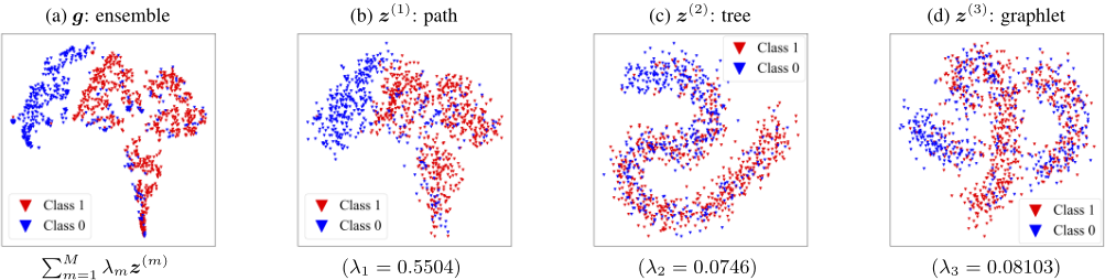
We conduct supervised XGL via pattern analysis, the proposed PXGL-GNN, by solving optimization (12) with the classification loss (10). The dataset is split into 80% training, 10% validation, and 10% testing data. The learned weight parameter λ, indicating each pattern's contribution to graph representation learning, is reported in Table 2. We also visualize the graph representation g and three pattern representations z(m) of PROTEINS in Figure 4. Results show the paths pattern is most important for learning g, and the ensemble representation g outperforms single pattern representations z(m) , which reveal underlying structural characteristics and naturally align with domain knowledge since paths are crucial for reflecting protein folding pathways [Yan et al., 2011].
The compared baselines include classical GNNs like GIN [Xu et al., 2018], DiffPool [Ying et al., 2018], DGCNN [Zhang et al., 2018], GRAPHSAGE [Hamilton et al., 2017]; subgraph-based GNNs like SubGNN [Kriege and Mutzel, 2012], SAN [Zhao et al., 2018], SAGNN [Zeng et al., 2023]; and recent methods like S2GAE [Tan et al., 2023] and ICL [Zhao et al., 2024]. The accuracies in Table 3 show that our method performs the best.
7.2 Unsupervised Learning
We conduct unsupervised XGL via pattern analysis, the proposed PXGL-GNN, by solving optimization (12) with the KL
| Pattern | MUTAG | PROTEINS | DD | NCI1 | COLLAB | IMDB-B | REDDIT-B | REDDIT-M5K |
|---|---|---|---|---|---|---|---|---|
| paths | 0.095 ±0.014 | 0.550±0.070 | 0.093 ±0.012 | 0.022 ±0.002 | 0.587±0.065 | 0.145 ±0.018 | 0.131 ±0.027 | 0.027 ±0.003 |
| trees | 0.046 ±0.005 | 0.074 ±0.009 | 0.054 ±0.006 | 0.063 ±0.008 | 0.105 ±0.013 | 0.022 ±0.003 | 0.055 ±0.007 | 0.025 ±0.003 |
| graphlets | 0.062 ±0.008 | 0.081 ±0.011 | 0.125 ±0.015 | 0.101 ±0.013 | 0.063 ±0.008 | 0.084 ±0.011 | 0.026 ±0.003 | 0.054 ±0.007 |
| cycles | 0.654±0.085 | 0.099 ±0.013 | 0.094 ±0.012 | 0.176 ±0.022 | 0.022 ±0.003 | 0.123 ±0.016 | 0.039 ±0.005 | 0.037 ±0.005 |
| cliques | 0.082 ±0.011 | 0.098 ±0.012 | 0.572±0.073 | 0.574±0.075 | 0.134 ±0.017 | 0.453±0.054 | 0.279 ±0.069 | 0.256 ±0.067 |
| wheels | 0.026 ±0.003 | 0.039 ±0.005 | 0.051 ±0.007 | 0.012 ±0.002 | 0.068 ±0.009 | 0.037 ±0.004 | 0.036 ±0.005 | 0.023 ±0.003 |
| stars | 0.035 ±0.005 | 0.056 ±0.007 | 0.011 ±0.002 | 0.052 ±0.007 | 0.021 ±0.003 | 0.136 ±0.017 | 0.447±0.006 | 0.578±0.033 |
| Method | MUTAG | PROTEINS | DD | NCI1 | COLLAB | IMDB-B | REDDIT-B | REDDIT-M5K |
|---|---|---|---|---|---|---|---|---|
| GIN | 84.53 ± 2.38 | 73.38 ±2.16 | 76.38 ±1.58 | 73.36 ±1.78 | 75.83 ± 1.29 | 72.52 ± 1.62 | 83.27 ± 1.30 | 52.48 ± 1.57 |
| DiffPool | 86.72 ± 1.95 | 76.07 ±1.62 | 77.42 ±2.14 | 75.42 ±2.16 | 78.77 ± 1.36 | 73.55 ± 2.14 | 84.16 ± 1.28 | 51.39 ± 1.48 |
| DGCNN | 84.29 ± 1.16 | 75.53 ±2.14 | 76.57 ±1.09 | 74.81 ±1.53 | 77.59 ± 2.24 | 72.19 ± 1.97 | 86.33 ± 2.29 | 53.18 ± 2.41 |
| GRAPHSAGE | 86.35 ± 1.31 | 74.21 ±1.85 | 79.24 ±2.25 | 77.93 ±2.04 | 76.37 ± 2.11 | 73.86 ± 2.17 | 85.59 ± 1.92 | 51.65 ± 2.55 |
| SubGNN | 87.52 ± 2.37 | 76.38 ±1.57 | 82.51 ±1.67 | 82.58 ±1.79 | 81.26 ± 1.53 | 71.58 ± 1.20 | 88.47 ± 1.83 | 53.27 ± 1.93 |
| SAN | 92.65 ± 1.53 | 75.62 ±2.39 | 81.36 ±2.10 | 83.07 ±1.54 | 82.73 ± 1.92 | 75.27 ± 1.43 | 90.38 ± 1.54 | 55.49 ± 1.75 |
| SAGNN | 93.24 ± 2.51 | 75.61 ±2.28 | 84.12 ±1.73 | 81.29 ±1.22 | 79.94 ± 1.83 | 74.53 ± 2.57 | 89.57 ± 2.13 | 54.11 ± 1.22 |
| ICL | 91.34 ± 2.19 | 75.44 ±1.26 | 82.77 ±1.42 | 83.45 ±1.78 | 81.45 ± 1.21 | 73.29 ± 1.46 | 90.13 ± 1.40 | 56.21 ± 1.35 |
| S2GAE | 89.27 ± 1.53 | 76.47 ±1.12 | 84.30 ±1.77 | 82.37 ±2.24 | 82.35 ± 2.34 | 75.77 ± 1.72 | 90.21 ± 1.52 | 54.53 ± 2.17 |
| PXGL-GNN | 94.87 ± 2.26 | 78.23 ±2.46 | 86.54 ±1.95 | 85.78 ±2.07 | 83.96 ± 1.59 | 77.35 ± 2.32 | 91.84 ± 1.69 | 57.36 ± 2.14 |
divergence loss (11). The learned weight parameter λ for XGL is reported in the supplementary materials. The visualizations of unsupervised XGL results are in the supplementary materials. Results show that the ensemble representation g outperforms single pattern representations z(m) .
For clustering performance, we use clustering accuracy (ACC) and Normalized Mutual Information (NMI). Baselines include four kernels: Randomwalk kernel (RW) [Borgwardt et al., 2005], Sub-tree kernels [Da San Martino et al., 2012], Graphlet kernels [Prˇzulj, 2007], Weisfeiler-Lehman (WL) kernels [Kriege and Mutzel, 2012]; and three unsupervised graph representation learning methods with Gaussian kernel in Eq. (11): InfoGraph [Sun et al., 2019], GCL [You et al., 2020], GraphACL [Luo et al., 2023]. The results are in Table 4 in our supplementary materials, and Table 5 reports the performance of PXGL-EGK. Our methods outperformed all benchmarks in almost all cases.
8 Conclusion
This paper investigates the explainability of graph representations through two novel approaches. First, we develop PXGL-EGK based on graph ensemble kernels that captures structural similarities while maintaining interpretability. Second, we introduce PXGL-GNN, a framework that incorporates diverse graph patterns (paths, trees, etc.) into GNNs to enhance both performance and explainability. We establish theoretical guarantees for our proposed methods, including robustness certification against perturbations and nonasymptotic generalization bounds. Extensive empirical evaluation demonstrates that our approaches not only achieve superior performance on classification and clustering tasks across multiple datasets, but also provide interpretable explanations for the learned graph representations.
Acknowledgements
This work was supported by the National Natural Science Foundation of China under Grant No.62376236, the Guangdong Provincial Key Laboratory of Mathematical Foundations for Artificial Intelligence (2023B1212010001), Shenzhen Science and Technology Program ZDSYS20230626091302006 (Shenzhen Key Lab of Multi-Modal Cognitive Computing), and Shenzhen Stability Science Program 2023.
Contribution Statement
Xudong Wang and Ziheng Sun contributed equally.
@inproceedings{ijcai2025p381,
  title     = {Explainable Graph Representation Learning via Graph Pattern Analysis},
  author    = {Wang, Xudong and Sun, Ziheng and Ding, Chris and Fan, Jicong},
  booktitle = {Proceedings of the Thirty-Fourth International Joint Conference on
               Artificial Intelligence, {IJCAI-25}},
  publisher = {International Joint Conferences on Artificial Intelligence Organization},
  editor    = {James Kwok},
  pages     = {3426--3434},
  year      = {2025},
  month     = {8},
  note      = {Main Track},
  doi       = {10.24963/ijcai.2025/381},
  url       = {https://doi.org/10.24963/ijcai.2025/381},
}
TY - CPAPER TI - Explainable Graph Representation Learning via Graph Pattern Analysis AU - Wang, Xudong AU - Sun, Ziheng AU - Ding, Chris AU - Fan, Jicong T2 - Proceedings of the Thirty-Fourth International Joint Conference on Artificial Intelligence, IJCAI-25 PB - International Joint Conferences on Artificial Intelligence Organization PY - 2025 SP - 3426 EP - 3434 DO - 10.24963/ijcai.2025/381 UR - https://doi.org/10.24963/ijcai.2025/381 ER -Copied
Machine-readable versions of this paper, for tools and AI agents:





