
Learning Neural Jump Stochastic Differential Equations with Latent Graph for Multivariate Temporal Point Processes
Proceedings of the Thirty-Fourth International Joint Conference on Artificial Intelligence. Main Track. Pages 3444-3452.
https://doi.org/10.24963/ijcai.2025/383
Keywords
- Data Mining: DM: Mining graphs
- Data Mining: DM: Mining spatial and/or temporal data
- Machine Learning: ML: Sequence and graph learning
- Data Mining: DM: Applications
Abstract
Multivariate Temporal Point Processes (MTPPs) play an important role in diverse domains such as social networks and finance for predicting event sequence data. In recent years, MTPPs based on Ordinary Differential Equations (ODEs) and Stochastic Differential Equations (SDEs) have demonstrated their strong modeling capabilities. However, these models have yet to thoroughly consider the underlying relationships among different event types to enhance their modeling capacity. Therefore, this paper introduces a method that uses neural SDEs with a jump process guided by the latent graph. Firstly, our proposed method employs multi-dimensional SDEs to capture the dynamics of the intensity function for each event type. Subsequently, a latent graph structure is integrated into the jump process without any encoder, aiming to enhance the modeling and predictive capabilities for MTPPs. Theoretical analysis guarantees the existence and uniqueness of the solution for our proposed method. The experiments conducted on multiple real-world datasets show that our approaches demonstrate significant competitiveness when compared to state-of-the-art neural point processes. Meanwhile, the trainable parameters of the latent graph also improve the model interpretability without any prior knowledge. Our code is available at https://github.com/cgao-comp/LNJSDE.
- [Chen et al., 2018] Ricky T. Q. Chen, Yulia Rubanova, Jesse Bettencourt, and David K Duvenaud. Neural ordinary dif- ferential equations. In Proceedings of the 32nd Interna- tional Conference on Neural Information Processing Sys- tems, volume 31, pages 6572-6583, 2018.
- [Daley and Vere-Jones, 2003] Daryl J Daley and David Vere-Jones. Basic properties of the poisson process. An Introduction to the Theory of Point Processes, 1:19-40, 2003.
- [Du et al., 2016] Nan Du, Hanjun Dai, Rakshit Trivedi, Utkarsh Upadhyay, Manuel Gomez-Rodriguez, and Le Song. Recurrent marked temporal point processes: Em- bedding event history to vector. In Proceedings of the 22nd ACM SIGKDD International Conference on Knowledge Discovery and Data Mining, pages 1555-1564, 2016.
- [Hawkes, 1971] Alan G Hawkes. Spectra of some self-exciting and mutually exciting point processes. Biometrika, 58(1):83-90, 1971.
- [Isham and Westcott, 1979] Valerie Isham and Mark West- cott. A self-correcting point process. Stochastic Processes and their Applications, 8(3):335-347, 1979.
- [Jia and Benson, 2019] Junteng Jia and Austin R Benson. Neural jump stochastic differential equations. Proceedings of the 33rd International Conference on Neural Informa- tion Processing Systems, pages 9847-9858, 2019.
- [Kingma and Ba, 2015] Diederik Kingma and Jimmy Ba. Adam: A method for stochastic optimization. In Proceed- ings of the 3rd International Conference on Learning Rep- resentations, 2015.
- [Kloeden et al., 1992] Peter E Kloeden, Eckhard Platen, Pe- ter E Kloeden, and Eckhard Platen. Stochastic Differential Equations. Springer, 1992.
- [Lemonnier et al., 2017] Rémi Lemonnier, Kevin Scaman, and Argyris Kalogeratos. Multivariate hawkes processes for large-scale inference. In Proceedings of the AAAI Con- ference on Artificial Intelligence, volume 31, pages 2168- 2174, 2017.
- [Mei and Eisner, 2017] Hongyuan Mei and Jason M Eisner. The neural hawkes process: A neurally self-modulating multivariate point process. Proceedings of the 31st In- ternational Conference on Neural Information Processing Systems, 30:6757-6767, 2017.
- [Meng et al., 2024] Zizhuo Meng, Ke Wan, Yadong Huang, Zhidong Li, Yang Wang, and Feng Zhou. Interpretable transformer hawkes processes: Unveiling complex interac- tions in social networks. In Proceedings of the 30th ACM SIGKDD Conference on Knowledge Discovery and Data Mining, pages 2200-2211, 2024.
- [Oh et al., 2024] YongKyung Oh, Dongyoung Lim, and Sungil Kim. Stable neural stochastic differential equations in analyzing irregular time series data. In Proceedings of the 12th International Conference on Learning Represen- tations, 2024.
- [Omi et al., 2019] Takahiro Omi, Kazuyuki Aihara, et al. Fully neural network based model for general temporal point processes. In Proceedings of the 33rd International Conference on Neural Information Processing Systems, volume 32, pages 2122-2132, 2019.
- [Pan et al., 2024] Liming Pan, Cheng Shi, and Ivan Dok- manic. A graph dynamics prior for relational inference. In Proceedings of the 38th AAAI Conference on Artificial Intelligence, volume 38, pages 14508-14516, 2024.
- [Pei et al., 2022] Hongbin Pei, Bo Yang, Jiming Liu, and Kevin Chen-Chuan Chang. Active surveillance via group sparse bayesian learning. IEEE Transactions on Pat- tern Analysis and Machine Intelligence, 44(3):1133-1148, 2022.
- [Reinhart, 2018] Alex Reinhart. A review of self-exciting spatio-temporal point processes and their applications. Statistical Science, 33(3):299-318, 2018.
- [Shchur et al., 2019] Oleksandr Shchur, Marin Biloš, and Stephan Günnemann. Intensity-free learning of temporal point processes. In Proceedings of the 7th International Conference on Learning Representations, 2019.
- [Song et al., 2024] Yujee Song, LEE Donghyun, Rui Meng, and Won Hwa Kim. Decoupled marked temporal point process using neural ordinary differential equations. In Proceedings of the 12th International Conference on Learning Representations, 2024.
- [Tung et al., 2016] Kuan-Chieh Tung, En Tzu Wang, and Ar- bee LP Chen. Mining event sequences from social me- dia for election prediction. In Proceedings of the 16th Industrial Conference on Data Mining, pages 266-281. Springer, 2016.
- [Yang and Zha, 2024] Sikun Yang and Hongyuan Zha. A variational autoencoder for neural temporal point pro- cesses with dynamic latent graphs. In Proceedings of the 38th AAAI Conference on Artificial Intelligence, vol- ume 38, pages 16343-16351, 2024.
- [Yang et al., 2022] Chenghao Yang, Hongyuan Mei, and Ja- son Eisner. Transformer embeddings of irregularly spaced events and their participants. In Proceedings of the 10th International Conference on Learning Representations, 2022.
- [Yoon et al., 2023] Kanghoon Yoon, Youngjun Im, Jingyu Choi, Taehwan Jeong, and Jinkyoo Park. Learning mul- tivariate hawkes process via graph recurrent neural net- work. In Proceedings of the 29th ACM SIGKDD Inter- national Conference on Knowledge Discovery and Data Mining, pages 5451-5462, 2023.
- [Zhang and Yan, 2021] Yunhao Zhang and Junchi Yan. Neu- ral relation inference for multi-dimensional temporal point processes via message passing graph. In Proceedings of the 30th International Joint Conference on Artificial Intel- ligence, pages 3406-3412, 2021. IJCAI
- [Zhang et al., 2020] Qiang Zhang, Aldo Lipani, Omer Kir- nap, and Emine Yilmaz. Self-attentive hawkes process. In Proceedings of the 37th International Conference on Ma- chine Learning, pages 11183-11193. PMLR, 2020.
- [Zhang et al., 2021] Qiang Zhang, Aldo Lipani, and Em- ine Yilmaz. Learning neural point processes with latent graphs. In Proceedings of the 30th Web Conference, pages 1495-1505, 2021.
- [Zhang et al., 2024] Shuai Zhang, Chuan Zhou, Yang Aron Liu, Peng Zhang, Xixun Lin, and Zhi-Ming Ma. Neural jump-diffusion temporal point processes. In Proceedings of the 41st International Conference on Machine Learn- ing, volume 235, pages 60541-60557. PMLR, 2024.
- [Zhou et al., 2013] Ke Zhou, Hongyuan Zha, and Le Song. Learning social infectivity in sparse low-rank networks us- ing multi-dimensional hawkes processes. In Proceedings of the 16th International Conference on Artificial Intelli- gence and Statistics, pages 641-649. PMLR, 2013.
- [Zuo et al., 2020] Simiao Zuo, Haoming Jiang, Zichong Li, Tuo Zhao, and Hongyuan Zha. Transformer hawkes pro- cess. In Proceedings of the 37th International Conference on Machine Learning, pages 11692-11702. PMLR, 2020.
References were extracted automatically from the PDF and may contain errors.
Full text extracted automatically from the PDF; figures, tables and equations may differ. The PDF is the version of record.
1 Introduction
Event data typically consists of extensive asynchronous event sequences, playing a crucial role across various domains from scientific research to industrial applications, underscoring its undeniable importance. Each event within these sequences is characterized by a timestamp and a type mark, indicating both when and what the event occurred. For instance, in seismology, advancements in technology have enabled the collection of large-scale earthquake event data, aiding scientists in better understanding and predicting seismic activities [Reinhart, 2018]. In financial, financial transaction records serve as event data widely utilized for detecting anomalies and forecasting market trends [Du et al., 2016]. On social media platforms, capturing social interaction data provides valuable insights, assisting in understanding user behavior and conducting sentiment analysis [Tung et al., 2016]. Temporal Point Processes (TPPs) represent a crucial tool for studying event sequences, primarily focusing on the occurrence times of events and the time intervals between events. Furthermore, for event sequences with multiple types of events, multivariate TPPs (MTPPs) can be applied to reveal the correlations, patterns, and trends among different event types.
∗Corresponding author.
The traditional TPPs typically rely on certain assumptions when defining the intensity function. For instance, the Hawkes process defines a self-exciting process indicating that
rences [Hawkes, 1971]. The self-correcting process assumes that the occurrence of past events inhibits the occurrence of future events [Isham and Westcott, 1979]. In a Poisson point process, the probability of an event occurring at each time point is constant and independent of past events [Daley and Vere-Jones, 2003]. These traditional TPP models provide a foundational framework for studying event sequences, but they also share some common limitations. These limitations include simplifying assumptions about the correlations between events, oversimplification of the dynamic evolution of event sequences, and ignoring complex patterns and nonlinear relationships. Consequently, in recent years, methods based on the powerful representational capabilities of neural networks have gradually emerged.
Due to advancements in deep learning, Neural Point Processes (NPPs) have gained significant attention for employing neural networks to model the intricate dynamics of asynchronous event sequences. For instance, Omi et al. introduce a fully neural network-based method to model the integral of the intensity function and obtain the intensity function as its derivative [Omi et al., 2019]. Shchur et al. propose an intensity-free method that learns without explicitly modeling the intensity function, reducing reliance on specific forms [Shchur et al., 2019]. Then, transformerbased approaches are proposed to use attention mechanisms to model MTPPs [Zuo et al., 2020]. However, these approaches still exhibit limitations when modeling continuoustime processes, particularly in terms of ensuring continuity and smoothness. Consequently, techniques rooted in Ordinary Differential Equations (ODEs) and Stochastic Differential Equations (SDEs) have showcased competitive performance [Song et al., 2024; Zhang et al., 2024]. Nevertheless, these methods do not explore the impact of underlying relationships between events, whereas graphs play a crucial role in predicting the spatiotemporal evolution of complex systems [Pei et al., 2022]. Therefore, the main motivation of this paper is to enhance the modeling capability of MTPPs by incorporating a latent graph over different types of events.
This paper presents a novel jump-diffusion SDE method with a latent graph for modeling MTPPs. Firstly, inspired by the equivalent SDE formulation of the multivariate Hawkes process, multi-dimensional SDEs are proposed to represent the hidden state of the intensity function of each event type. Then, we integrate an encoder-free graph representation method and design interaction functions between events in the jump process to capture potential relationships between events, which can further enhance the representation and predictive abilities of event sequences. Moreover, the proof of existence and uniqueness of solutions enhances the reliability of our approach.
Our main contributions are as follows:
- Multi-dimensional SDEs are employed to model the intensity function for each event type, enhancing the representation capability of the underlying MTPPs.
- To further capture the underlying relationships between events, a graph generator without encoders is incorporated. Subsequently, interaction functions between event types in the jump process are also proposed.
- We prove the existence and uniqueness of the solutions of our approach. Meanwhile, experimental results show that the performance of our approach is better than other SOTA methods.
2 RelatedWorks
2.1 Neural Point Processes
Due to certain limitations in traditional TPPs, such as the definition of intensity functions or kernel functions, NPPs have gradually become a focus of research. Early methods are mainly based on Recurrent Neural Networks (RNNs) to model point processes by assuming a specific functional form for the time evolution of the intensity function of a point process [Du et al., 2016; Mei and Eisner, 2017]. To overcome this limitation, Omi et al. propose a method that directly models the cumulative hazard by neural networks and obtains the intensity function with the automatic differentiation techniques [Omi et al., 2019]. Subsequently, several methods have been proposed that leverage Transformer architecture networks to capture the dependencies between events [Zuo et al., 2020; Zhang et al., 2020; Yang et al., 2022; Meng et al., 2024]. With the development of neural ODEs and SDEs, methods based on modeling continuous systems rather than other architectures like RNNs can explicitly model the smooth transitions between states of intensity functions [Chen et al., 2018]. Jia et al. propose NJSDE, a neural ODEs-based hybrid system that encompasses both flow and jump processes, to model TPPs [Jia and Benson, 2019]. Song et al. introduce Dec-ODE to decouple the hidden state dynamics by neural ODEs [Song et al., 2024]. Zhang et al. present NJDTPP, where the intensity process is designed by a neural jump-diffusion SDE [Zhang et al., 2024]. It is worth noting that both NJSDE and NJDTPP also design the impact of event occurrences in their jump items. However, neither of them continues to deeply consider the underlying relationships between event types. Consequently, this oversight may lead to the magnification of the impact between unrelated events. Furthermore, NJSDE uses ODEs to model the overall system rather than each event type, while NJDTPP employs one-dimensional SDEs for each event type. In contrast, our innovative approach utilizes multidimensional SDEs to capture more complex temporal dynamics for each event type. These improvements enhance the predictive and modeling capabilities of our approach.
2.2 Temporal Point Processes with Graph
In traditional TPPs, besides establishing a probabilistic graphical model based on existing knowledge, some methods aim to infer relationships among events. For instance, Zhou et al. propose a method to infer latent connectives between users in social networks by a multivariate Hawkes process [Zhou et al., 2013]. Lemonnier et al. propose a Low-Rank Hawkes Process framework for fitting multivariate Hawkes processes in large-scale problems [Lemonnier et al., 2017]. With the emergence of NPPs, some NPPs models combining graphs have appeared. Zhang et al. adopt a variational inference framework to model the posterior relation of MTPP data for probabilistic estimation [Zhang and Yan, 2021]. Zhang et al. propose a probabilistic graph generator. The sampled graph can be easily integrated as a plug-in to modify an existing NPP model [Zhang et al., 2021]. Yoon et al. extract potential graph structures through data processing and encode multivariate event sequences into a sequence of graphs, enhancing the predictive capability of the model [Yoon et al., 2023]. Yang et al. partition event sequences into different sub-intervals based on prior knowledge and establish dynamic graph relationships using a Variational Autoencoder (VAE) to capture changes in relationships between different event types [Yang and Zha, 2024]. In a nutshell, NPPs with latent graphs have effectively enhanced the interpretability and predictive capability of the model. However, SDE-based methods have not yet explored this aspect, which is also the motivation of our method.
3 Preliminaries
3.1 Multivariate Point Processes
A MTPP is a stochastic process that describes the temporal evolution of multiple event types V = {1, 2, ..., V }, where V is the number of event types. Let S = {(vi, ti)}Li=1 be an event sequence, where the tuple (vi, ti) is the i-th event, vi ∈ V and ti ∈ [0, T] are its event type and timestamp, T is the size of the time window. A general MTPP can be characterized by the conditional intensity function of each event type k ∈ V:
where dNk(t) = Nk(t +∆t) -Nk(t) ∈ {0, 1} is the jump size, Nk(t) counts the number of the event type k prior to history H(t) until time t, H(t) = {(v′ , t′ )|t′ < t, v′ ∈ V} records the history. The log-likelihood of observing a sequence S is the sum of the log-likelihood of events and nonevents and can be expressed as Eq. (2). The optimization of MTPPs is to maximize the log-likelihood.
3.2 Multivariate Hawkes Processes
We then introduce a classic and important MTPP known as the Multivariate Hawkes Process (MHP). Let N(t) = (N1(t), . . . , NV (t))T be a MTPP, where its intensity function λk(t) for each event type k is defined as follows:
where µk ∈ R+ represents the base intensity, and g(t) ∈ R+ denotes a kernel function that signifies the extent of influence of an event. The entry αjk indicates how event type j effects event type k.
3.3 Stochastic Differential Equations
A basic SDE can be defined as:
where x0 is the initial value, f is the drift coefficient function, g is the diffusion coefficient function, {W(t)}t≥0 is a Brownian motion. Then, X={X(t)}t≥0 is called a solution of the SDE, and it satisfies the Itˆo integral equation.
In the context of neural SDEs, the selection of the diffusion function is especially crucial. To make training stable, this paper also considers a Linear Noise SDE (LNSDE) [Oh et al., 2024], presented as follows.
It has been proved that, with appropriate neural network designs, the LNSDEs in Eq. (6) have their unique strong solutions. Furthermore, neural LNSDEs also demonstrate robustness in maintaining excellent performance and effectively preventing overfitting.
3.4 Equivalent SDE Formulation for MHPs
To establish a connection between SDEs and MTPPs, the following derived equivalent SDE formulation is introduced.
Theorem 1. Suppose that the kernel function g(t) = exp(-β(t)), the MHPs N(t) and its intensity functions
λ(t) = (λ1(t), . . . , λV (t))T can be equivalently expressed as the solution to the jump SDEs. Each λk(t) follows
Proof. The proof is similar to the univariate Hawkes Process discussed in [Zhang et al., 2024], which can be found in Appendix A.1.
4 Methodologies
4.1 Overview
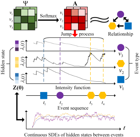
As shown in Fig. 1, the proposed method involves SDEs with jumps designed for MTPPs with a latent graph. To better capture the internal states within each event, every event type is associated with multidimensional hidden states that evolve according to an SDE system. Moreover, we employ a graph generator without any encoder and integrate the influence of the latent graph into the jump process.
4.2 Proposed SDEs for Intensity function
Due to the diversity of underlying dynamical systems, we introduce two different variants of SDEs for the hidden state in our model as Eqs. (8) and (9), which denote whether the diffusion term is time-independent or not. In our model design, we assume that each type of event k ∈ V has its corresponding hidden state Zk, and Zk(t) evolves as a SDE. To more accurately capture the temporal effects, the continuous SDE between events [ti-1, ti) is designed as follows:
where f : RdZ × R+ × R+ → RdZ considers not only the hidden state Zk(t) but also the time ti-1 and the time since the last event occurred t - ti-1, while the diffusion term g : RdZ → RdZ is dependent on the hidden state Zk(t), {Wk(t)}t≥0 is a dZ-dimensional Brownian motion. Also, the version of neural LNSDE can be expressed as follows.
where the function g : R+ → RdZ is dependent on the time t-ti-1. For the convenience of discussion, we use Eq. (8) as the default. Furthermore, the proposed approach can directly adopt Eq. (6).
Then, the intensity function λk(t) of each event type k is defined as follows.
where η : RdZ → R, softplus(x) = log(1 + exp(ζx))/ζ ensures the λk(t) > 0 and ζ is a hyper-parameter.
4.3 Latent Graph in Jump Process
From Theorem 1, it can be intuitively observed that the influence between different types of events takes effect when events occur. Therefore, compared to incorporating the effects of node interactions into the drift coefficient function, our proposed approach emphasizes the latent relationships between different types of events in the jump process. Moreover, this method can reduce computational costs by passing messages between nodes solely at the times of event occurrences, rather than continuously throughout all time.
Firstly, let us consider the situation without any graph structure. In this case, the occurrence of an event of one type will have a certain impact on all other types of events. Therefore, when an event type j occurs at time t, then the jump size ∆Zk(t) = Zk(t+)-Zk(t) of event type k can be formulated as Eq. (11).
where t+ is the right-limit of t, the function ρ : RdZ ×RdZ → RdZ is used to capture the interaction between different types of events. Furthermore, in general, the form of the jump size can be extended as
However, our proposed approach incorporates a latent graph in the jump process to emphasize capturing potential relationships between event types. Trying to capture events that are practically unrelated may result in a decrease in the model's representation and predictive capabilities. Therefore, we adopt a method to integrate a latent graph without an encoder inspired by [Pan et al., 2024]. Additionally, we design interaction functions to enhance the model's ability to capture relationships between different event types.
The latent graph 1 is constructed as follows.
where a ∈ {0, 1}, Ψ0 and Ψ1 ∈ R are trainable parameters, and γ is the inverse temperature, and A1 = 11T - A0 . Instead of using the initial states Z(0) to build the latent graph, this way can decouple the graph structure from the hidden states to enhance training stability, especially when dealing with long sequences.
Then, the jump size of event k is designed by incorporating the latent graph as shown in Eq. (14).
where ˆ Zjk(t) is the interaction term between event type vj and vk under the latent graph, ρv : RdZ → RdZ is the jumpwise function, ρn : RdZ × RdZ → RdZ is the aggregationwise function and ρe(a) : RdZ ×RdZ → RdZ is the edge-wise function for adjacency matrix Aa .
4.4 Theoretical Analysis
Based on the two sections mentioned above, our proposed approach can be expressed as follows.
where Z(t)=(Z1(t), ...,ZV (t))T is a collection of latent state vectors, W(t)=(W1(t), ...,WV (t))T is a collection of Brownian motions, its components Wv(t) are pairwise independent, ∆Z(t)=(∆Z1(t), ...,∆ZV (t))T are calculated by Eq. (14), t and ti-1 are also column vectors. We then proceed to investigate the existence and uniqueness of the solution {Z(t)}t≥0 and {λ(t)}t≥0 to our proposed approach.
Theorem 2. Assuming that f , g, ρv , ρn , ρe , η are measurable functions and satisfy the Lipschitz continuity condition, ρv , ρn , ρe are continuous, then a strong unique solution Z := {Z(t)}t≥0 exists, once initial values z := {zk}Vk=1 is fixed, and the resulting process λ := {λ(t)}t≥0 also has a strong unique solution.
1 In this context, the term "graph relationships" does not refer to the ground-truth causal relationships but rather to Granger causality, which aims to assess the utility of one variable in predicting other variables.
4.5 Model Training
Throughout the training process, we utilize the EulerMaruyama scheme [Kloeden et al., 1992] with a constant step size for its computational efficiency. This scheme subdivides the time interval (ti-1, ti] into D sub-intervals, where ti-1=τ i0<· · · <τ id<· · · <τ iD=ti with the fixed step size ∆id = (ti - ti-1)/D. Then, for each hidden state Zk, Eq. (8) on (ti-1, ti] can be discredited by the recursive equation as Eq. (16).
for d ∈ {0, 1, ..., D - 1}, and Zk(τ i0 ) = Zk(t+i-1 ), ∆W i d = W(τ id+1 ) -W(τ id ) is sampled fromN(0,∆id ) for numerical computation. Finally, the log-likelihood can be approximated as follows.
where τ 1 0 =0, τ L+1 D =T, λk(t) can be calculated by Eqs. (10) and (15).
4.6 Time and Event Prediction
To predict the subsequent event time and event type based on the historical events H(ti), the conditional density function of the next event time for ˆ ti+1 ≥ ti is estimated as Eq. (18).
where λ(t) = ∑Vk=1 λk(t).
For the next event type prediction ˆ vi+1, it can be estimated by Eq. (19).ˆ vi+1 = argmaxk∈V λk(ti+1)/λ(ti+1). (19)
5 Experiments
5.1 Datasets
We evaluate our proposed approaches and other baselines on five real-world benchmark datasets used in [Yang and Zha, 2024; Zhang et al., 2024], including New York Motor Vehicle Collisions (NYMVC), two stack exchange datasets (MathOF and AskUbuntu), Taobao and Taxi. The statistical characteristics of these datasets are shown in Table 1. Additionally, to scale down the time, a logarithmic transformation is applied to all time values. We also ensure that at most one event occurs at any given time to facilitate the training and prediction processes for all models. More detailed information of datasets can be found in Appendix B.
| Datasets | Train | Dev | Test | Events | Average length | Types |
|---|---|---|---|---|---|---|
| NYMVC | 120 | 40 | 40 | 12736 | 63.68 | 5 |
| MathOF | 156 | 52 | 52 | 50464 | 194.09 | 15 |
| AskUbuntu | 102 | 34 | 35 | 31194 | 182.42 | 11 |
| Taobao | 1300 | 200 | 500 | 115397 | 57.69 | 17 |
| Taxi | 1400 | 200 | 400 | 74078 | 37.04 | 10 |
5.2 Baselines
We compare our approaches with the following eight state-ofthe-art models. One RNN-based model: Recurrent Marked Temporal Point Process (RMTPP) [Du et al., 2016]. One TPP with fully neural networks (FullyNN) [Omi et al., 2019]. Two attention-based models: Transformer Hawkes Process (THP) [Zuo et al., 2020], Attentive Neural Hawkes Process (AttNHP) [Yang et al., 2022] and Interpretable Transformer Hawkes Processes (ITHP) [Meng et al., 2024]. One log-normal mixture distribution-based model: Variational Autoencoder for MTPPs with Dynamic Latent Graphs (VAETPP) [Yang and Zha, 2024]. One ODEs-based method: (NJSDE) [Jia and Benson, 2019]. One SDEs-based method: Neural Jump-Diffusion Temporal Point Processes (NJDTPP) [Zhang et al., 2024]. The detailed description and comparison of baselines can be found in Appendix C.
5.3 Experimental Settings
For our approaches, both f and g in our approach are implemented as three-layer Multilayer Perceptions (MLPs), which contain an input layer, a hidden layer, and an output layer. In the jump process, ρv , ρn , and ρe are two-layer MLPs, each consisting of an input layer and an output layer. The activation function default used is Tanh. The dimension dZ of Z is set to 32, and the dimension of hidden layers is uniformly set to 64. The learning rate of parameters in neural networks is set to 0.001 for the NYMVC dataset and 0.0001 for other datasets, and the learning rate of initial hidden states z and Ψ is set to 0.1. We employ the Adam optimizer [Kingma and Ba, 2015] to optimize the parameters. During the training process, the number of sub-intervals D in the Euler-Maruyama scheme is set to 10, while during the prediction process, D is set to 1000 for a more precise forecast. More details can be found in Appendix D. As for the other comparative baselines, their settings are adopted from the original papers.
5.4 EvaluationMetrics
We utilize the negative log-likelihood (NLL) as a metric to assess the modeling capability of event sequences in real-world datasets. Furthermore, we assess performance in the standard next-event prediction task within TPPs, predicting each subsequent event (vi, ti) based on the history H(ti). Event time prediction is evaluated using Root Mean Square Error (RMSE), while event type prediction is assessed through accuracy and the weighted F1 score. The accuracy in multiclass classification represents the proportion of correct classifications. The weighted F1 score provides a better assessment of class imbalance situations. These metrics are shown in Eqs. (20), (21) and (22).
| Dataset | NYMVC | Mathof | AskUbuntu | Taobao | Taxi | |||||
|---|---|---|---|---|---|---|---|---|---|---|
| Metric | NLL | RMSE | NLL | RMSE | NLL | RMSE | NLL | RMSE | NLL | RMSE |
| RMTPP | 1.647 | 0.825 | 1.891 | 0.753 | 1.776 | 0.443 | 1.659 | 0.533 | 0.227 | 0.373 |
| FullyNN | 1.172 | 0.844 | 1.399 | 0.655 | 1.525 | 0.573 | 1.489 | 0.574 | 0.310 | 0.366 |
| NJSDE | 0.655 | - | 0.508 | - | 1.505 | - | -0.342 | - | -0.392 | - |
| THP | -0.642 | 0.336 | -0.532 | 0.872 | -0.508 | 0.355 | 1.191 | 0.531 | 0.442 | 0.373 |
| AttNHP | -0.632 | 0.108 | -0.427 | 0.181 | -0.585 | 0.236 | 1.206 | 0.530 | 0.491 | 0.369 |
| ITHP | -1.053 | - | -0.845 | - | -1.106 | - | 0.465 | - | -0.362 | - |
| VAETPP | -0.886 | 0.0596 | -0.822 | 0.136 | -1.016 | 0.111 | -1.064 | 0.120 | -0.592 | 0.311 |
| NJDTPP | -0.764 | 0.0948 | -1.058 | 0.160 | -1.922 | 0.154 | -0.474 | 0.132 | -0.293 | 0.296 |
| Our SDE | -0.961 | 0.0837 | -1.512 | 0.132 | -2.186 | 0.127 | -0.979 | 0.193 | -0.595 | 0.284 |
| Our LNSDE | -0.991 | 0.0787 | -1.571 | 0.126 | -2.200 | 0.129 | -1.000 | 0.198 | -0.580 | 0.284 |
| Dataset | NYMVC | Mathof | AskUbuntu | Taobao | Taxi | |||||
|---|---|---|---|---|---|---|---|---|---|---|
| Metric | Accuracy | F1 | Accuracy | F1 | Accuracy | F1 | Accuracy | F1 | Accuracy | F1 |
| RMTPP | 0.241 | 0.186 | 0.154 | 0.127 | 0.189 | 0.163 | 0.431 | 0.429 | 0.836 | 0.815 |
| FullyNN | 0.244 | 0.199 | 0.166 | 0.132 | 0.245 | 0.188 | 0.440 | 0.410 | 0.812 | 0.782 |
| NJSDE | 0.298 | 0.145 | 0.136 | 0.08 | 0.227 | 0.108 | 0.430 | 0.264 | 0.644 | 0.615 |
| THP | 0.291 | 0.226 | 0.211 | 0.183 | 0.315 | 0.249 | 0.467 | 0.406 | 0.865 | 0.828 |
| AttNHP | 0.315 | 0.231 | 0.173 | 0.103 | 0.289 | 0.177 | 0.458 | 0.386 | 0.761 | 0.724 |
| ITHP | 0.285 | 0.213 | 0.239 | 0.221 | 0.352 | 0.323 | 0.602 | 0.577 | 0.911 | 0.886 |
| VAETPP | 0.320 | 0.236 | 0.234 | 0.191 | 0.341 | 0.225 | 0.573 | 0.442 | 0.866 | 0.832 |
| NJDTPP | 0.304 | 0.212 | 0.254 | 0.211 | 0.358 | 0.311 | 0.486 | 0.452 | 0.908 | 0.891 |
| Our SDE | 0.354 | 0.311 | 0.281 | 0.261 | 0.394 | 0.364 | 0.611 | 0.598 | 0.925 | 0.913 |
| Our LNSDE | 0.382 | 0.348 | 0.298 | 0.282 | 0.391 | 0.358 | 0.610 | 0.593 | 0.924 | 0.911 |
where C denotes the number of classes, wi denotes the sample weight for class i, and F1i represents the F1 score for class i.
5.5 Experimental Results
In Table 2, the performance of the baselines and our proposed methods is presented in terms of negative log-likelihood and time prediction RMSE on various datasets. Concerning NLL, our proposed approaches consistently achieve some of the highest rankings across all datasets, showcasing the robust modeling capabilities of our approach for MTPPs. NJDTPP and VAETPP also demonstrate commendable performance. In the realm of time prediction, our proposed methods and VAETPP exhibit strong competitiveness. VAETPP utilizes a mixture of log-normal distributions to model the distribution of one-dimensional inter-event times, enhancing its capability for time prediction. Consequently, its time prediction accuracy leads on some datasets, while our approaches also perform well on the majority of datasets.
Table 3 illustrates the accuracy of predicting event types using various methods on real-world datasets. The results indicate that our methods, SDE and LNSDE variants, outperform other baselines in terms of prediction accuracy across all datasets, underscoring the effectiveness of our methods tailored for MTPPs. One reason for the lower accuracy of event prediction in NJSDE is that it models the entire system based on ODEs, making it difficult to accurately represent the hidden states of each event. Furthermore, SDE and LNSDE variants demonstrate varying performances across different datasets, highlighting the importance of careful consideration when selecting diffusion terms. Suitable diffusion term selections will further enhance prediction accuracy. Additionally, the competitive performance of VAETPP and NJDTPP is also noteworthy. The discernible gap between accuracy and weighted F1 arises from the imbalance in event categories, particularly evident in the AskUbuntu dataset.
Overall, our proposed methods have demonstrated strong capabilities in modeling, time prediction, and event-type prediction on various real-world datasets, further illustrating the effectiveness of our proposed methods.
5.6 Ablation Study
Our ablation experiments are designed as follows: ODE-NA signifies that the version of our approach without both the Brownian motion and the latent graph in the jump process, as depicted in Eq. (11). The ρ function is also implemented through three-layer MLPs. ODE denotes the version of our approach without Brownian motion.
| Dataset | Taobao | AskUbuntu | ||||||
|---|---|---|---|---|---|---|---|---|
| Variants | NLL | RMSE | Acc | F1 | NLL | RMSE | Acc | F1 |
| ODE-NA | -0.855 | 0.279 | 0.600 | 0.583 | -2.088 | 0.130 | 0.360 | 0.316 |
| ODE | -0.956 | 0.216 | 0.605 | 0.585 | -2.170 | 0.129 | 0.374 | 0.332 |
| SDE | -0.979 | 0.193 | 0.611 | 0.598 | -2.186 | 0.127 | 0.394 | 0.364 |
| LNSDE | -1.000 | 0.198 | 0.610 | 0.593 | -2.200 | 0.129 | 0.391 | 0.358 |
The results shown in Table 4 show that the performance is significantly improved by incorporating a latent graph in the jump process. This also demonstrates that considering the dependency levels among different event types can enhance the modeling and predictive capabilities of the model. Furthermore, utilizing SDE will further enhance the accuracy of modeling and prediction.
5.7 Hyperparameter Analysis
Number of Sub-intervals
For the solver of SDEs (e.g., Euler-Maruyama method in our approach), a large number of sub-intervals results in a more accurate approximation of the integral but also linearly increases the time complexity. Following our preliminary experiments, we generally found that there is a good balance between training time and effectiveness when the number of sub-intervals D=10. For instance, the impacts on our LNSDE variant on NYMVC are in Table 5.
| D | NLL | RMSE | Accuracy | F1 | Sec/Epoch |
| 5 | -0.984 | 0.0824 | 0.380 | 0.344 | 2.409 |
| 10 | -0.991 | 0.0787 | 0.382 | 0.348 | 4.247 |
| 15 | -0.993 | 0.0772 | 0.383 | 0.348 | 6.871 |
Dimensions of Hidden State Zk(t)
We also conduct experiments regarding the dimensions of the hidden state Zk(t). For instance, the performances of our LNSDE variant on NYMVC and Mathof are in Table 6.
| Dataset | NYMVC | Mathof | ||||||
|---|---|---|---|---|---|---|---|---|
| |Zk(t)| | NLL | RMSE | Acc | F1 | NLL | RMSE | Acc | F1 |
| 8 | -0.842 | 0.081 | 0.312 | 0.223 | -1.053 | 0.133 | 0.217 | 0.181 |
| 16 | -0.896 | 0.082 | 0.325 | 0.276 | -1.356 | 0.128 | 0.256 | 0.227 |
| 32 | -0.961 | 0.083 | 0.354 | 0.311 | -1.512 | 0.132 | 0.281 | 0.261 |
| 64 | -1.104 | 0.096 | 0.403 | 0.380 | -1.682 | 0.134 | 0.309 | 0.296 |
The results show that increasing the dimensionality provides significant improvement in predicting events. However, overly large dimensions can harm time prediction, since the model may memorize noise or over-fit instead of capturing true temporal patterns.
5.8 Model Interpretability
The learned latent dependencies among events can offer some interpretability to the model. As a result, we conduct an experiment on a synthetic network to present the interpretability of our model.
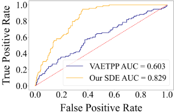
We initially create a directed graph with 20 nodes. Then, we simulate a multivariate Hawkes process 100 times. Here, the parameters µ and α are randomly sampled from uniform distributions U[0, 0.02] and U[0.1, 0.3], respectively, while the time delays follow an exponential distribution with a parameter of β = 2.5. After training, we acquire the edge probabilities in the same way in [Pan et al., 2024]. Subsequently, we compare these edge probabilities to the groundtruth graph structure by the Receiver Operating Characteristic (ROC) curve, and the Area under the ROC Curve (AUC) value. Furthermore, we conduct similar testing on the static version of VAETPP, a SOTA NPPs model with a latent graph. As shown in Fig. 2, the AUC obtained by our approach is better than VAETPP, indicating a more precise capture of the latent relationships between different event types. More detailed information can be found in Appendix E.
6 Conclusion
In this study, we propose a novel approach that leverages multi-dimensional SDEs to enhance the representation capability of the underlying MTPPs. Additionally, we incorporate a graph generator to capture the dependency structure between event types and improve the interaction function between event types in the jump process. Theoretical analysis proves the existence and uniqueness of the solutions of our proposed approaches. Furthermore, experimental results have demonstrated that our method outperforms state-of-theart methods in terms of modeling ability and prediction performance. In the future, we aim to expand the scope of our research by extending our model to encompass the dynamics of non-stationary networks and addressing the scalability of NPPs in larger-scale data, especially concerning the largescale latent graph.
Acknowledgements
This research was supported by the National Natural Science Foundation of China (Nos. 62261136549, 62471403, U22A2098, 62271411), the Technological Innovation Team of Shaanxi Province (No. 2025RS-CXTD-009), the International Cooperation Project of Shaanxi Province (No. 2025GH-YBXM-017), the Fundamental Research Funds for the Central Universities (Nos. G2024WD0151, D5000240309).
@inproceedings{ijcai2025p383,
  title     = {Learning Neural Jump Stochastic Differential Equations with Latent Graph for Multivariate Temporal Point Processes},
  author    = {Wang, Yuchen and Hou, Dongpeng and Gao, Chao and Li, Xianghua},
  booktitle = {Proceedings of the Thirty-Fourth International Joint Conference on
               Artificial Intelligence, {IJCAI-25}},
  publisher = {International Joint Conferences on Artificial Intelligence Organization},
  editor    = {James Kwok},
  pages     = {3444--3452},
  year      = {2025},
  month     = {8},
  note      = {Main Track},
  doi       = {10.24963/ijcai.2025/383},
  url       = {https://doi.org/10.24963/ijcai.2025/383},
}
TY - CPAPER TI - Learning Neural Jump Stochastic Differential Equations with Latent Graph for Multivariate Temporal Point Processes AU - Wang, Yuchen AU - Hou, Dongpeng AU - Gao, Chao AU - Li, Xianghua T2 - Proceedings of the Thirty-Fourth International Joint Conference on Artificial Intelligence, IJCAI-25 PB - International Joint Conferences on Artificial Intelligence Organization PY - 2025 SP - 3444 EP - 3452 DO - 10.24963/ijcai.2025/383 UR - https://doi.org/10.24963/ijcai.2025/383 ER -Copied
Machine-readable versions of this paper, for tools and AI agents:





