
Let’s Group: A Plug-and-Play SubGraph Learning Method for Memory-Efficient Spatio-Temporal Graph Modeling
Proceedings of the Thirty-Fourth International Joint Conference on Artificial Intelligence. Main Track. Pages 3471-3479.
https://doi.org/10.24963/ijcai.2025/386
Keywords
- Multidisciplinary Topics and Applications: MTA: Sensor networks and smart cities
- Machine Learning: ML: Time series and data streams
- Machine Learning: ML: Applications
- Data Mining: DM: Mining spatial and/or temporal data
Abstract
Spatio-temporal graph modeling is widely applied to spatio-temporal data, analyzing the relationships between data to achieve accurate predictions. However, despite the excellent predictive performance of increasingly complex models, their intricate architectures result in significant memory overhead and computational complexity when handling spatio-temporal data, which limits their practical applications. To address these challenges, we propose a plug-and-play SubGraph Learning (SGL) method to reduce the memory overhead without compromising performance. Specifically, we introduce a SubGraph Partition Module (SGPM), which leverages a set of learnable memory vectors to select node groups with similar features from the graph, effectively partitioning the graph into smaller subgraphs. Noting that partitioning the graph may lead to feature redundancy, as overlapping information across subgraphs can occur. To overcome this, we design a SubGraph Feature Aggregation Module (SGFAM), which mitigates redundancy by averaging node features from different subgraphs. Experiments on four traffic network datasets of various scales demonstrate that SGL can significantly reduce memory overhead, achieving up to a 56.4\% reduction in average GPU memory overhead, while maintaining robust prediction performance. The source code is available at https://github.com/wengwenchao123/SubGraph-Learning.
- [Bai et al., 2020] Lei Bai, Lina Yao, Can Li, Xianzhi Wang, and Can Wang. Adaptive graph convolutional recurrent network for traffic forecasting. Advances in neural infor- mation processing systems, 33:17804-17815, 2020.
- [Deng et al., 2024] Jiewen Deng, Renhe Jiang, Jiaqi Zhang, and Xuan Song. Multi-modality spatio-temporal forecast- ing via self-supervised learning. In Kate Larson, editor, Proceedings of the Thirty-Third International Joint Con- ference on Artificial Intelligence, IJCAI-24, pages 2018- 2026. International Joint Conferences on Artificial Intelli- gence Organization, 8 2024. Main Track. IJCAI
- [Dong et al., 2024] Zheng Dong, Renhe Jiang, Haotian Gao, Hangchen Liu, Jinliang Deng, Qingsong Wen, and Xuan Song. Heterogeneity-informed meta-parameter learning for spatiotemporal time series forecasting. In Proceedings of the 30th ACM SIGKDD conference on knowledge dis- covery and data mining, pages 631-641, 2024.
- [Fan et al., 2024] Jin Fan, Wenchao Weng, Qikai Chen, Huifeng Wu, and Jia Wu. Pdg2seq: Periodic dynamic graph to sequence model for traffic flow prediction. Neural Networks, page 106941, 2024.
- [Fang et al., 2023] Yuchen Fang, Yanjun Qin, Haiyong Luo, Fang Zhao, and Kai Zheng. Stwave+: A multi-scale ef- ficient spectral graph attention network with long-term trends for disentangled traffic flow forecasting. IEEE Transactions on Knowledge and Data Engineering, 2023.
- [Fang et al., 2024] Yuchen Fang, Yuxuan Liang, Bo Hui, Zezhi Shao, Liwei Deng, Xu Liu, Xinke Jiang, and Kai Zheng. Efficient large-scale traffic forecasting with trans- formers: A spatial data management perspective. arXiv preprint arXiv:2412.09972, 2024.
- [Gao et al., 2024] Haotian Gao, Renhe Jiang, Zheng Dong, Jinliang Deng, Yuxin Ma, and Xuan Song. Spatial- temporal-decoupled masked pre-training for spatiotempo- ral forecasting. In Kate Larson, editor, Proceedings of the Thirty-Third International Joint Conference on Arti- ficial Intelligence, IJCAI-24, pages 3998-4006. Interna- tional Joint Conferences on Artificial Intelligence Orga- nization, 8 2024. Main Track.
- [Guo et al., 2019] Shengnan Guo, Youfang Lin, Ning Feng, Chao Song, and Huaiyu Wan. Attention based spatial- temporal graph convolutional networks for traffic flow forecasting. In Proceedings of the AAAI conference on artificial intelligence, volume 33, pages 922-929, 2019.
- [Guo et al., 2021] Shengnan Guo, Youfang Lin, Huaiyu Wan, Xiucheng Li, and Gao Cong. Learning dynamics and heterogeneity of spatial-temporal graph data for traffic forecasting. IEEE Transactions on Knowledge and Data Engineering, 34(11):5415-5428, 2021.
- [Guo et al., 2023] Shengnan Guo, Youfang Lin, Letian Gong, Chenyu Wang, Zeyu Zhou, Zekai Shen, Yiheng Huang, and Huaiyu Wan. Self-supervised spatial-temporal bottleneck attentive network for efficient long-term traffic forecasting. In 2023 IEEE 39th International Conference on Data Engineering (ICDE), pages 1585-1596. IEEE, 2023.
- [He et al., 2025] Kecheng He, Hongjie Jia, Yunfei Mu, Xi- aodan Yu, Yue Zhou, Jianzhong Wu, and Xiaohong Dong. Leasing business model for trunk mobile charging sta- tions: From the view of operators. IEEE Transactions on Transportation Electrification, 2025.
- [Jiang et al., 2023a] Jiawei Jiang, Chengkai Han, Wayne Xin Zhao, and Jingyuan Wang. Pdformer: Propagation delay- aware dynamic long-range transformer for traffic flow pre- diction. In Proceedings of the AAAI conference on artifi- cial intelligence, volume 37, pages 4365-4373, 2023.
- [Jiang et al., 2023b] Renhe Jiang, Zhaonan Wang, Jiawei Yong, Puneet Jeph, Quanjun Chen, Yasumasa Kobayashi, Xuan Song, Shintaro Fukushima, and Toyotaro Suzumura. Spatio-temporal meta-graph learning for traffic forecast- ing. In Proceedings of the AAAI conference on artificial intelligence, volume 37, pages 8078-8086, 2023.
- [Karypis and Kumar, 1998] George Karypis and Vipin Ku- mar. A fast and high quality multilevel scheme for parti- tioning irregular graphs. SIAM Journal on scientific Com- puting, 20(1):359-392, 1998.
- [Lee and Ko, 2024] Hyunwook Lee and Sungahn Ko. Tes- tam: A time-enhanced spatio-temporal attention model with mixture of experts. In The Twelfth International Con- ference on Learning Representations, 2024.
- [Li and Zhu, 2021] Mengzhang Li and Zhanxing Zhu. Spatial-temporal fusion graph neural networks for traffic flow forecasting. In Proceedings of the AAAI conference on artificial intelligence, volume 35, pages 4189-4196, 2021.
- [Li et al., 2018] Yaguang Li, Rose Yu, Cyrus Shahabi, and Yan Liu. Diffusion convolutional recurrent neural net- work: Data-driven traffic forecasting. In International Conference on Learning Representations, 2018.
- [Li et al., 2023] Fuxian Li, Jie Feng, Huan Yan, Guangyin Jin, Fan Yang, Funing Sun, Depeng Jin, and Yong Li. Dynamic graph convolutional recurrent network for traffic prediction: Benchmark and solution. ACM Transactions on Knowledge Discovery from Data, 17(1):1-21, 2023.
- [Liu et al., 2023] Hangchen Liu, Zheng Dong, Renhe Jiang, Jiewen Deng, Jinliang Deng, Quanjun Chen, and Xuan Song. Spatio-temporal adaptive embedding makes vanilla transformer sota for traffic forecasting. In Proceedings of the 32nd ACM international conference on information and knowledge management, pages 4125-4129, 2023.
- [Liu et al., 2024] Xu Liu, Yutong Xia, Yuxuan Liang, Jun- feng Hu, Yiwei Wang, Lei Bai, Chao Huang, Zhenguang Liu, Bryan Hooi, and Roger Zimmermann. Largest: A benchmark dataset for large-scale traffic forecasting. Ad- vances in Neural Information Processing Systems, 36, 2024.
- [Qin et al., 2023] Yanjun Qin, Haiyong Luo, Fang Zhao, Yuchen Fang, Xiaoming Tao, and Chenxing Wang. Spatio- temporal hierarchical mlp network for traffic forecasting. Information Sciences, 632:543-554, 2023.
- [Shao et al., 2022a] Zezhi Shao, Zhao Zhang, Fei Wang, and Yongjun Xu. Pre-training enhanced spatial-temporal graph neural network for multivariate time series forecasting. In Proceedings of the 28th ACM SIGKDD conference on knowledge discovery and data mining, pages 1567-1577, 2022.
- [Shao et al., 2022b] Zezhi Shao, Zhao Zhang, Wei Wei, Fei Wang, Yongjun Xu, Xin Cao, and Christian S Jensen. De- coupled dynamic spatial-temporal graph neural network for traffic forecasting. Proceedings of the VLDB Endow- ment, 15(11):2733-2746, 2022.
- [Shen et al., 2025] Zekai Shen, Haitao Yuan, Xiaowei Mao, Congkang Lv, Shengnan Guo, Youfang Lin, and Huaiyu Wan. Towards an efficient and effective en route travel time estimation framework. arXiv preprint arXiv:2504.04086, 2025.
- [Van der Maaten and Hinton, 2008] Laurens Van der Maaten and Geoffrey Hinton. Visualizing data using t-sne. Journal of machine learning research, 9(11), 2008.
- [Wang et al., 2024a] Binwu Wang, Pengkun Wang, Zhengyang Zhou, Zhe Zhao, Wei Xu, and Yang Wang. Make bricks with a little straw: Large-scale spatio- temporal graph learning with restricted gpu-memory capacity. In Kate Larson, editor, Proceedings of the Thirty-Third International Joint Conference on Artificial Intelligence, IJCAI-24, pages 2388-2396. International Joint Conferences on Artificial Intelligence Organization, 8 2024. Main Track.
- [Wang et al., 2024b] Hongjun Wang, Jiyuan Chen, Tong Pan, Zheng Dong, Lingyu Zhang, Renhe Jiang, and Xuan Song. Robust traffic forecasting against spatial shift over years. arXiv preprint arXiv:2410.00373, 2024.
- [Weng et al., 2023] Wenchao Weng, Jin Fan, Huifeng Wu, Yujie Hu, Hao Tian, Fu Zhu, and Jia Wu. A decomposition dynamic graph convolutional recurrent network for traffic forecasting. Pattern Recognition, 142:109670, 2023.
- [Weng et al., 2024] Wenchao Weng, Mei Wu, Hanyu Jiang, Wanzeng Kong, Xiangjie Kong, and Feng Xia. Pattern- matching dynamic memory network for dual-mode traffic prediction. arXiv preprint arXiv:2408.07100, 2024.
- [Wu et al., 2019] Zonghan Wu, Shirui Pan, Guodong Long, Jing Jiang, and Chengqi Zhang. Graph wavenet for deep spatial-temporal graph modeling. In Proceedings of the Twenty-Eighth International Joint Conference on Artificial Intelligence. International Joint Conferences on Artificial Intelligence Organization, 2019. IJCAI
- [Xia et al., 2022] Mengran Xia, Dawei Jin, and Jingyu Chen. Short-term traffic flow prediction based on graph convolu- tional networks and federated learning. IEEE Transactions on Intelligent Transportation Systems, 24(1):1191-1203, 2022.
- [Zeng et al., 2025] Hansheng Zeng, Yuqi Li, Ruize Niu, Chuanguang Yang, and Shiping Wen. Enhancing spatiotemporal prediction through the integration of mamba state space models and diffusion transformers. Knowledge-Based Systems, 2025.
- [Zhang et al., 2024] Yudong Zhang, Pengkun Wang, Binwu Wang, Xu Wang, Zhe Zhao, Zhengyang Zhou, Lei Bai, and Yang Wang. Adaptive and interactive multi-level spatio-temporal network for traffic forecasting. IEEE Transactions on Intelligent Transportation Systems, 2024.
- [Zhao et al., 2023] Yusheng Zhao, Xiao Luo, Wei Ju, Chong Chen, Xian-Sheng Hua, and Ming Zhang. Dynamic hy- pergraph structure learning for traffic flow forecasting. In 2023 IEEE 39th International Conference on Data Engi- neering (ICDE), pages 2303-2316. IEEE, 2023.
- [Zheng et al., 2020] Chuanpan Zheng, Xiaoliang Fan, Cheng Wang, and Jianzhong Qi. Gman: A graph multi- attention network for traffic prediction. In Proceedings of the AAAI conference on artificial intelligence, volume 34, pages 1234-1241, 2020.
References were extracted automatically from the PDF and may contain errors.
Full text extracted automatically from the PDF; figures, tables and equations may differ. The PDF is the version of record.
1 Introduction
In recent years, advances in data collection and processing capabilities have generated large volumes of high-quality spatio-temporal data (e.g., weather conditions, traffic status) [Wang et al., 2024b; Zeng et al., 2025; Shen et al., 2025; He et al., 2025], which have been widely applied in related research fields. Due to its spatio-temporal correlations can be effectively captured by Spatio-Temporal Graph Neural Networks (STGNNs) [Wu et al., 2019; Jiang et al., 2023b; Deng et al., 2024], these learning algorithms have emerged as the dominant approach for spatio-temporal data modeling tasks.
∗ corresponding Author.
Existing STGNNs typically take spatio-temporal sequences collected by nodes (e.g., traffic segments, weather stations) as input and model them as spatio-temporal graphs to extract features (e.g., through graph convolution or attention mechanisms) [Shao et al., 2022b; Jiang et al., 2023a; Guo et al., 2023]. Early STGNNs utilized geographic information to construct graph structure [Li et al., 2018], but these methods neglected the hidden spatio-temporal relationships in the data, leading to suboptimal performance. As a result, recent studies generally focus on capturing relationships through dynamic construction of spatio-temporal graphs, followed by feature extraction from the data [Weng et al., 2023; Li et al., 2023; Dong et al., 2024]. However, these approaches have high computational complexity, resulting in substantial GPU memory overhead for STGNNs [Liu et al., 2023]. In addition, as the number of nodes increases, the memory overhead of STGNNs grows significantly, which limits the realworld applications [Wang et al., 2024a; Liu et al., 2024].
In this paper, we aim to address the challenge of spatiotemporal graph modeling under limited GPU memory constraints. One intuitive solution is to partition the spatiotemporal graph into smaller subgraphs, extract features from these subgraphs, and then aggregate node features across the subgraphs to learn the features of the entire spatio-temporal graph. This approach effectively reduces the originally high computational complexity to a manageable level, thereby saving GPU memory. However, the partitioning of the spatiotemporal graph presents a challenge. Existing partitioning methods typically rely on static partitioning, without considering the dynamic nature of the spatio-temporal graph. For example, PatchSTG [Fang et al., 2024] uses the geographical coordinates of nodes to partition subgraphs, while FCGCN [Xia et al., 2022] employs the Louvain algorithm to partition subgraphs based on the topological relationships among nodes. However, all of these methods fail to capture complex spatio-temporal dependencies.
For the above challenges, we propose a plug-and-play SubGraph Learning (SGL) method. Specifically, we design a SubGraph Partition Module (SGPM), which can be directly integrated into existing spatio-temporal graph models to partition the graph and significantly reduce the memory overhead required by the model. SGPM employs a set of learnable memory vectors as anchors and selects the most similar group of nodes in the spatiot-emporal graph as subgraphs by calculating the similarity between node features and memory vector features. This approach partitions the spatio-temporal graph into multiple smaller subgraphs and uses these subgraphs to extract node features, thus drastically reducing computational complexity and significantly lowering the GPU memory overhead.
At the same time, the way processing each divided subgraph separately solves the memory overhead and complexity problem. However, it brings a potential risk of feature redundancy. Therefore, we subsequently design a SubGraph Feature Aggregation Module (SGFAM) to eliminate it. Specifically, SGAM firstly extracts features of the node from different subgraphs it has appeared, and then averages these features. According to these operations, the node feature is more balanced and completeness. Overall, our contributions are as follows:
- We propose a plug-and-play SubGraph Learning (SGL) method to reduce the memory overhead required by existing models. SGL uses a SubGraph Partition Module (SGPM), which partitions the spatio-temporal graph into multiple subgraphs for feature extraction, effectively reducing the model's computational complexity and significantly lowering the computational cost.
- We introduce a SubGraph Feature Aggregation Module (SGFAM). This module efficiently integrates the feature of nodes across various subgraphs, avoiding redundancy in node feature and improving the completeness of spatio-temporal graph feature representation.
- We evaluate the effectiveness of SGL on traffic datasets of different scales. Experimental results show that our proposed method can effectively reduce the computational cost while maintaining model performance, with a maximum average GPU memory overhead reduction of 56.4%.
2 RelatedWork
Spatio-temporal graph construction. As the key component of spatio-temporal graph models, spatio-temporal graph construction has attracted significant attention from researchers. DCRNN [Li et al., 2018] uses predefined matrix based on road segment distances as spatio-temporal graphs. AGCRN [Bai et al., 2020] generates adaptive graphs using adaptive embeddings to learn the correlations between nodes. STFGNN [Li and Zhu, 2021] constructs a Spatial-Temporal Fusion Graph using the FastDTW algorithm to extract local correlations. Attention mechanisms also play a crucial role in spatio-temporal graph learning. For example, PDformer [Jiang et al., 2023a] uses DTW and predefined matrix as mask matrix to calculate the weights of the graph structure. STWave [Fang et al., 2023] constructs a local graph attention network using predefined matrix to efficiently model spatial correlations. LarSTL [Wang et al., 2024a] uses the METIS
algorithm [Karypis and Kumar, 1998] and geographic coordinates to partition the traffic road network into multiple subgraphs for continuous learning. However, these methods still model spatio-temporal graphs with static relationships, without accounting for the dynamic nature of spatio-temporal graphs.
Spatio-temporal graph neural networks. In recent years, with the rise of deep learning, Spatio-Temporal Graph Neural Networks (STGNNs) have emerged as one of the most representative methods for capturing spatio-temporal dependencies , becoming a rising star in the field of spatio-temporal graph modeling. For example, GMAN [Zheng et al., 2020] uses a transformed attention mechanism to reduce biases between the past and the future. STAEformer [Liu et al., 2023] introduces spatio-temporal adaptive embedding to enhance the performance of Transformers. DyHSL [Zhao et al., 2023] designs a dynamic hypergraph learning method to capture the dynamic and complex relationships in traffic networks. PDG2Seq [Fan et al., 2024] leverages periodic information to generate dynamic graphs and utilizes an RNN-based iterative prediction method to capture future trend changes. Additionally, some studies have approached model performance enhancement from other perspectives. For instance, STEP [Shao et al., 2022a] and STD-MAE [Gao et al., 2024] enhance performance by designing pre-training models to generate rich contextual representations that can seamlessly integrate with any architecture. EXPERT [Lee and Ko, 2024] proposes a novel Mixture of Experts (MoE) framework, which generates new graphs based on evolving environmental conditions to address the issue of spatial distribution drift during testing. However, these methods come with substantial computational overhead despite enhancing accuracy.
3 Method
In this section, we first provide the mathematical definition of the problem studied in this paper. Next, we introduce the feature extraction process of spatial feature extraction modules commonly used in current spatio-temporal graph models. Finally, we explain in detail the working principles of SGPM and SGFAM and how they integrate into existing models.
3.1 Spatio-Temporal GraphModeling
A spatio-temporal graph is represented by G = (V, E), where V is the set of nodes and E is the set of edges representing the adjacency relationships between road segments. At time point t, the historical feature data of graph G can be represented as Xt = {x1t , x2t , ..., xNt } ∈ RN×d , where xit represents the traffic conditions of node i at time t, d represents the number of features, N is the number of nodes.
We aim to learn a spatio-temporal prediction model g() that can effectively predict the feature data for the next Q time steps using the historical feature data from the past P time steps, X = {X1, ..., XP } ∈ RP×N×d . The goal is to predict the future data Y = {XP+1, ..., XP+Q} ∈ RQ×N×d :
3.2 Spatio-Temporal Graph Feature Extraction
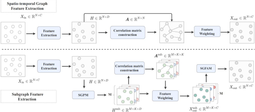
In existing STGNNs, spatio-temporal graph features are typically extracted using graph convolution or attention mechanisms [Guo et al., 2021]. As shown in Figure 1, the spatiotemporal graph feature extraction process can be divided into three steps.
First, feature extraction is applied to each node, mapping its original features into the latent space and enhancing the node representations. It can be represented as:
where Xin ∈ RN×C represents the input spatio-temporal data, H ∈ RN×D represents the extracted hidden features, and Fin is the feature extraction function used to extract the hidden features from the spatio-temporal data. This function can be implemented using methods like MLP, among others.
According to spatio-temporal characteristics of each node, the correlation matrix construction module then represents the relationships among nodes in the graph. This can be expressed as:
where A ∈ RN×N represents the correlation matrix between nodes, and G() is the method for constructing the correlation matrix. This can be achieved using techniques such as dynamic graph construction or attention score matrix construction.
Finally, the feature weighting module enhances the representations of each node through the spatiotemporal correlation matrix extracted by the previous step. This process can be expressed as:
where Hout ∈ RN×C represents the extracted spatiotemporal graph features, Fout() transforms the extracted features into a format suitable for input to the next layer.
From the above formulas, it can be seen that the complexity of spatio-temporal graph feature extraction is highly dependent on the number of nodes N.
3.3 SubGraph Partition
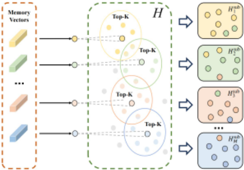
The limited GPU memory capacity imposes restrictions on the scale of the input graph. To address this challenge, we propose a SubGraph Partition Module (SGPM). As shown in Figure 1, SGPM is placed after the feature extraction function and partitions the spatio-temporal graph into multiple smaller subgraphs based on similarity. By extracting features from these subgraphs separately, this approach reduces the GPU memory capacity required.
As shown in Figure 2, SGPM uses a set of randomly initialized memory vectors P = [P1, P2, ..., PM] ∈ RM×D as anchors to construct subgraphs.
Specifically, we first compute the similarity between each memory vector Pi and the node features H, which can be represented as:
where wi ∈ RN×1 represents the similarity between the memory vector Pi and the node features H.
Since highly correlated nodes tend to have similar features, Pi can serve as an anchor point to select nodes with higher similarity, forming a subgraph, which can be expressed as:
where idxi ∈ RK represents the indices of the top K nodes with the highest similarity to Pi. Using idxi, we collect the corresponding nodes and their features to form a subgraph, which can be represented as:
thus, a subgraph is obtained for each memory vector, and the related subgraph indices and feature sets can be represented as: idx = {idx1, ..., idxM} ∈ RM×K , and Hsub = {Hsub 1 , ...,H sub M } ∈ RM×K×D .
3.4 Subgraph Feature Extraction
Similar to the general spatio-temporal graph feature extraction methods, each subgraph extracts the features between its nodes by constructing a correlation matrix, represented as:
where Asub i ∈ RK×K represents the correlation matrix of subgraph i, and all subgraphs share the same G(). The collection of correlation matrices for all subgraphs is denoted as Asub = {Asub 1 , ...,Asub M } ∈ RM×K×K .
Finally, the spatial features of the subgraph nodes are extracted by multiplying the node features of the subgraph with the correlation matrix:
where Hsub out ∈ RM×K×C represents the spatio-temporal graph features extracted from the subgraph.
3.5 SubGraph Feature Aggregation
As shown in Figure 1, we propose a SubGraph Feature Aggregation Module (SGFAM), placed after the feature weighting layer, to integrate node features from different subgraphs. As shown in Figure 3, we use the subgraph indices idx to collect the features of the same nodes across different subgraphs. This process can be expressed as:
where Hi represents the set of features for node i extracted from all subgraphs. To ensure a more comprehensive representation of the extracted features, we average these features to obtain the final output feature, expressed as:
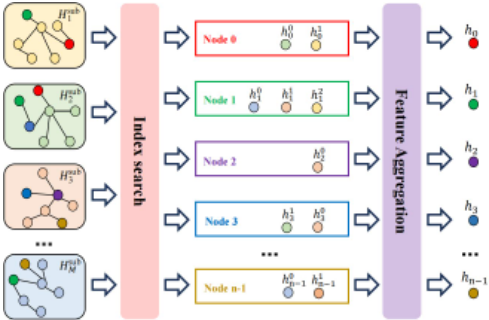
where Hiout ∈ RN×D is the final hidden feature for node i, sum() represents the sum of features in Hi , and count() denotes the number of features in Hi .
Finally, the aggregated hidden features for all nodes are represented as:
where Hout ∈ RN×C represents the final output of SGFAM.
3.6 Complexity Analysis
In traditional spatio-temporal graph feature extraction, the complexity is tightly coupled with the number of nodes N due to the construction of the correlation matrix and the feature weighting process. For instance, both graph convolution and attention mechanisms have a complexity of O(N 2 ). In contrast, under the subgraph learning approach, spatiotemporal feature extraction consists mainly of three components: subgraph partitioning, correlation matrix construction, and node feature aggregation. The complexities of these components are as follows: subgraph partitioning is O(NM +MK), correlation matrix construction is O(K2 ) (since subgraphs are computed in parallel), and node feature aggregation is O(MK+N). Thus, the overall complexity of spatio-temporal feature extraction using the subgraph learning approach is O(NM + MK + K2 + N). Since M is significantly smaller than K and N, it can be considered a constant, simplifying the complexity to O(N +K2 ). When K is considerably smaller than N, the computational complexity of the subgraph learning method is significantly lower than that of the traditional spatio-temporal graph feature extraction methods, leading to a substantial reduction in memory consumption.
4 Experiment
To evaluate the performance of our proposed SGL, we selecte a series of representative spatio-temporal models that utilize dynamic graph convolution or attention mechanisms to extract spatial features. We integrate SGPM and SGFAM into their spatial feature extraction modules for subgraph partitioning and feature aggregation to assess the effectiveness of SGPM and SGFAM. In this work, we aim to address the following questions:
- Q1: How do SGL and dynamic graph convolution or attention mechanisms in different backbone networks perform in terms of spatio-temporal graph modeling tasks, efficiency, and memory overhead?
- Q2: Are SGPM and SGFAM effective?
- Q3: How sensitive is SGPM to the number of subgraphs and the number of nodes per subgraph?
- Q4: What are the characteristics of the nodes in the subgraphs divided by SGPM?
Backbones To validate the effectiveness of SGL, we select a series of models based on graph convolution and attention mechanisms to extract spatial features as backbones for the experiments. These models can be categorized into two types based on their computation methods: 1) Parallel Computation Models: GMAN [Zheng et al., 2020], STWavefull GAT [Fang et al., 2023], STWave-ESGAT [Fang et al., 2023], STAEformer [Liu et al., 2023], DGCNet(P) [Weng et al., 2024]; 2) Serial Computation Models: DGCRN [Li et al., 2023], DDGCRN [Weng et al., 2023], DGCNet(R) [Weng et al., 2024].
Dataset We select four widely-used real-world traffic datasets (PEMS03, PEMS04, PEMS07, and PEMS08) [Guo et al., 2019; Li and Zhu, 2021] for a series of experiments to investigate the performance, efficiency, and memory overhead differences of SGL across various backbone networks' spatial feature extraction modules in traffic prediction tasks. These experiments aim to evaluate SGL in scenarios with different node scales: small-scale (PEMS08), medium-scale (PEMS03, PEMS04), and large-scale (PEMS07). The detailed information for each dataset is provided in Table 1.
| Datasets | Nodes | Time steps | Time range |
|---|---|---|---|
| PEMS03 | 358 | 26208 | 09/01/2018 - 11/30/2018 |
| PEMS04 | 307 | 16992 | 01/01/2018 - 02/28/2018 |
| PEMS07 | 883 | 28224 | 05/01/2017 - 08/31/2017 |
| PEMS08 | 170 | 17856 | 07/01/2016 - 08/31/2016 |
Experimental Setup Following the settings from previous studies [Guo et al., 2019; Li and Zhu, 2021], we divide the datasets into training, validation, and test sets in a 6:2:2 ratio based on the time order. Our experiments are conducted on a GPU server equipped with a GeForce GTX 4090 graphics card, using the PyTorch framework. All models, including their SGL variants, strictly follow the original training configurations to ensure fair comparison, including optimizers, maximum training epochs, and early stop strategies. For the PEMS07 dataset, the batch size is set to 16, while the batch size for the other three datasets is set to 64. The settings for the number of subgraphs M and the number of nodes per subgraph K for each dataset are detailed in Table 2.
To comprehensively evaluate the performance of SGL , we assess it from three aspects:
| dataset | PEMS03 | PEMS04 | PEMS07 | PEMS08 | ||||
|---|---|---|---|---|---|---|---|---|
| M | K | M | K | M | K | M | K | |
| DGCNet(P)-SGL | 4 | 100 | 4 | 80 | 10 | 100 | 4 | 50 |
| DGCNet(R)-SGL | 4 | 100 | 4 | 80 | 10 | 100 | 4 | 60 |
| DDGCRN-SGL | 4 | 100 | 4 | 80 | 10 | 100 | 4 | 50 |
| STAEformer-SGL | 4 | 100 | 4 | 80 | 10 | 100 | 4 | 50 |
| DGCRN-SGL | 4 | 100 | 4 | 80 | 10 | 100 | 4 | 60 |
| GMAN-SGL | 4 | 100 | 4 | 80 | 10 | 100 | 4 | 50 |
| STWave-SGL | 4 | 100 | 4 | 80 | 10 | 100 | 4 | 50 |
- Performance Evaluation: We use three evaluation metrics: Mean Absolute Error (MAE), Mean Absolute Percentage Error (MAPE), and Root Mean Squared Error (RMSE).
- Memory Overhead: We use GPU cost as a metric.
- Running Efficiency: We evaluate using train time and inference time as metrics.
4.1 Performance and Effciency Analysis (Q1)
Table 3 shows the prediction performance, efficiency, and memory overhead of each model and its SGL variant. From the table, we observe that the models and their SGL variants achieve comparable prediction performance, but the SGL variants significantly reduce memory overhead, demonstrating the effectiveness of the SGL method.
On datasets of varying scales, as the dataset size increases, the memory savings of SGL become more pronounced. For instance, under identical conditions on the small-scale PEMS08 dataset, the memory overhead of DDGCRN-SGL is reduced by 18.2% compared to DDGCRN. On the large-scale PEMS07 dataset, DDGCRN-SGL reduces memory overhead by 60.5% compared to DDGCRN, highlighting the practicality of SGL's divide-and-conquer subgraph partitioning strategy. Although STWave-ESGAT can also reduce memory overhead while maintaining performance, it requires predefined matrix to determine the attention range, which may not be applicable in certain situations. On the other hand, STWave-SGL does not have this limitation, making it more versatile.
Regarding operational efficiency, models like GMAN, representing parallel computation frameworks, fully leverage parallel processing in their SGL variants, significantly accelerating computation speeds. In contrast, serial computation models like DGCRN, which rely on RNNs for iterative feature extraction, do not achieve parallel computation. Nevertheless, their SGL variants maintain comparable operational efficiency to their prototypes while demonstrating superior efficiency when the number of nodes is large.
4.2 Ablation Experiment (Q2)
SubGraph Partitioning Method To verify the rationality of SGPM, we design two alternative subgraph partitioning methods and one node clustering-based feature extraction method and test them on DGCNet(R) to demonstrate the effectiveness of our proposed SGPM:
| dataset | PEMS03 | PEMS04 | |||||||||||
|---|---|---|---|---|---|---|---|---|---|---|---|---|---|
| MAE | RMSE | MAPE | GPUCost (GB) | train time (s/epoch) | inference time (s) | MAE | RMSE | MAPE | GPUCost (GB) | train time (s/epoch) | inference time (s) | ||
| DGCRN DGCRN-SGL | 14.67 14.69 | 26.08 25.19 | 14.65% 15.01% | 11.68 9.64 | 106.95 125.32 | 16.05 20.64 | 18.73 18.71 | 30.59 30.44 | 12.80% 13.02% | 9.46 7.75 | 56.45 80.77 | 7.62 11.47 | |
| DDGCRN DDGCRN-SGL | 14.63 14.54 | 25.11 25.03 | 14.61% 14.89% | 8.86 5.22 | 30.2 36.31 | 3.30 4.67 | 18.41 18.40 | 30.69 30.47 | 12.27% 12.21% | 6.95 4.04 | 18.42 20.3 | 1.88 2.66 | |
| DGCNet(R) DGCNet(R)-SGL | 14.88 14.85 | 25.30 25.43 | 15.32% 14.61% | 8.92 5.21 | 36.47 35.96 | 4.05 4.31 | 18.35 18.49 | 30.48 30.75 | 12.23% 12.19% | 6.97 3.94 | 20.12 22.51 | 1.98 2.71 | |
| GMAN GMAN-SGL | 17.00 16.20 | 28.64 28.16 | 18.05% 16.48% | 12.32 7.51 | 51.09 32.49 | 9.30 4.53 | 18.77 18.77 | 31.09 30.99 | 12.37% 12.33% | 9.71 6.05 | 22.17 17.04 | 3.00 2.46 | |
| STWave-full GAT STWave-ESGAT STWave-SGL | 15.06 15.04 15.00 | 27.45 26.48 26.41 | 15.36% 15.36% 15.34% | 13.98 11.28 12.12 | 60.12 70.94 61.84 | 8.58 10.15 8.97 | 18.17 18.28 18.23 | 29.98 30.14 30.14 | 12.35% 12.24% 12.16% | 11.56 10.6 10.37 | 35.47 39.15 33.80 | 4.85 5.72 4.92 | |
| STAEformer STAEformer-SGL | 15.27 15.04 | 27.78 26.07 | 15.40% 15.10% | 19.46 14.94 | 79.03 68.80 | 8.63 7.67 | 18.25 18.29 | 29.94 30.27 | 12.09% 12.08% | 15.73 12.41 | 43.13 37.57 | 4.65 4.14 | |
| DGCNet(P) DGCNet(P)-SGL | 14.79 14.72 | 25.49 25.33 | 14.95% 15.09% | 9.83 5.54 | 31.81 23.38 | 3.61 3.32 | 18.26 18.32 | 30.96 30.68 | 12.20% 12.12% | 7.64 4.43 | 16.43 12.04 | 1.98 1.96 | |
| dataset PEMS07 | PEMS08 | ||||||||||||
| MAE | RMSE | MAPE | GPUCost (GB) | train time (s/epoch) | inference time (s) | MAE | RMSE | MAPE | GPUCost (GB) | train time (s/epoch) | inference time (s) | ||
| DGCRN DGCRN-SGL | 20.01 20.27 | 33.18 33.17 | 8.41% 8.53% | 11.43 6.06 | 418.3 472.45 | 47.8 67.83 | 14.27 14.38 | 23.42 23.49 | 9.36% 9.53% | 4.36 4.26 | 59.30 71.94 | 7.71 10.68 | |
| DDGCRN DDGCRN-SGL | 19.79 19.76 | 33.23 33.42 | 8.35% 8.38% | 12.59 4.97 | 274.63 148.81 | 28.62 16.49 | 14.4 14.35 | 23.84 23.66 | 9.34% 9.41% | 2.85 2.33 | 16.18 20.92 | 1.82 2.78 | |
| DGCNet(R) DGCNet(R)-SGL | 19.47 19.65 | 33.67 33.53 | 8.15% 8.22% | 12.51 4.79 | 278.17 145.53 | 30.03 18.16 | 13.69 13.66 | 23.46 23.38 | 8.98% 9.01% | 2.85 2.33 | 19.91 26.55 | 2.27 3.38 | |
| GMAN GMAN-SGL | 19.80 19.60 | 33.57 33.45 | 8.32% 8.23% | 16.22 4.71 | 166.77 80.48 | 20.71 11.31 | 14.32 14.22 | 24.61 24.33 | 9.44% 9.47% | 4.15 3.21 | 11.08 10.03 | 1.75 1.43 | |
| STWave-full GAT STWave-ESGAT STWave-SGL | 19.22 19.78 19.42 | 32.80 34.10 33.36 | 8.07% 8.20% 8.09% | 11.37 7.94 7.87 | 191.92 198.2 159.06 | 25.92 27.32 24.03 | 13.74 13.76 13.70 | 23.52 23.30 23.23 | 9.12% 9.11% 9.07% | 6.04 5.84 5.99 | 24.72 25.87 22.14 | 3.41 3.71 3.32 | |
| STAEformer | 19.22 | 32.72 | 8.04% | 22.11 | 306.91 | 33.69 20.88 | 13.48 | 23.27 | 8.83% 8.86% | 7.59 | 22.31 | 2.53 2.77 | |
| STAEformer-SGL | 19.16 | 32.53 | 8.04% | 9.34 | 181.66 | 27.59 | 13.44 13.95 | 23.35 23.99 | 9.29% | 6.54 | 22.14 9.23 | ||
| DGCNet(P) DGCNet(P)-SGL | 19.6 19.61 | 33.81 33.26 | 8.28% 8.28% | 12.81 4.31 | 253.56 76.04 | 11.42 | 13.694 | 23.64 | 9.09% | 3.09 2.34 | 10.88 | 1.43 1.68 | |
- DGCNet(R)-RD: This method randomly partitions the original traffic network into equally sized subgraphs for feature extraction.
- DGCNet(R)-METIS: This method uses the DTW algorithm to generate a similarity matrix for the nodes and then applies the METIS algorithm to partition the subgraphs.
- DGCNet(R)-DC: This method clusters node features into subgraph representations using a mapping matrix [Qin et al., 2023; Zhang et al., 2024] and then employs these subgraph cluster representations for spatio-temporal graph feature extraction.
| Dataset | PEMS04 | PEMS08 | ||||
|---|---|---|---|---|---|---|
| Metric | MAE | RMSE | MAPE | MAE | RMSE | MAPE |
| DGCNet(R)-SGL | 18.49 | 30.75 | 12.19% | 13.66 | 23.38 | 9.01% |
| DGCNet(R)-RD | 18.71 | 31.42 | 12.41% | 14.07 | 23.62 | 9.30% |
| DGCNet(R)-METIS | 18.68 | 31.23 | 12.24% | 13.91 | 23.81 | 9.15% |
| DGCNet(R)-DC | 18.90 | 31.35 | 12.92% | 14.34 | 23.85 | 9.89% |
Table 4 presents the performance of the three variants on PEMS08. We observe that the other two subgraph partitioning methods perform worse than SGPM. DGCNet(R)- RD generates subgraphs through random partitioning without considering node correlations, resulting in the poorest performance. DGCNet(R)-METIS constructs subgraphs where nodes exhibit high correlation by calculating similarities via dynamic programming, thus outperforming DGCNet(R)-RD. However, as the subgraphs in DGCNet(R)-METIS remain fixed and fail to account for the dynamic changes in node correlations, its performance is still inferior to DGCNet(R)- SGL. DGCNet(R)-DC utilizes a mapping matrix to transform node features into subgraph representations. However, this approach results in the loss of individual node features, which significantly hampers its performance compared to other methods.
Feature Aggregation Methods To validate the rationality of the averaging operation for feature aggregation, we design two alternative aggregation methods for comparison:
- DGCNet(R)-sum: This method directly uses the sum of node features instead of averaging them.
- DGCNet(R)-max: This method selects the maximum feature from the set of subgraph node features as the node's
final feature.
| Dataset | PEMS04 | PEMS08 | ||||
|---|---|---|---|---|---|---|
| Metric | MAE | RMSE | MAPE | MAE | RMSE | MAPE |
| DGCNet(R)-SGL | 18.49 | 30.75 | 12.19% | 13.66 | 23.38 | 9.01% |
| DGCNet(R)-max | 18.60 | 30.87 | 12.26% | 13.81 | 23.60 | 9.07% |
| DGCNet(R)-sum | 18.71 | 31.42 | 12.24% | 13.83 | 23.45 | 9.00% |
Figure 5 shows the performance of the three aggregation methods. It is evident that the averaging operation yields the best results. DGCNet(R)-sum suffers from feature redundancy, resulting in the poorest performance among the three variants. DGCNet(R)-max captures the most representative feature by selecting the largest feature as the node's feature but neglects feature from other subgraphs, leading to slightly worse performance than DGCNet(R)-SGL. These results demonstrate that the averaging operation avoids redundancy and proves its effectiveness in aggregating feature.
4.3 Hyperparameter Experiment (Q3)
We conduct hyperparameter experiments on the PEMS07 dataset using DDGCRN-SGL to evaluate the impact of the number of nodes per subgraph K and the number of subgraphs M on the model's predictive performance. Figure 4 illustrates the effect of K and M on the model's performance.
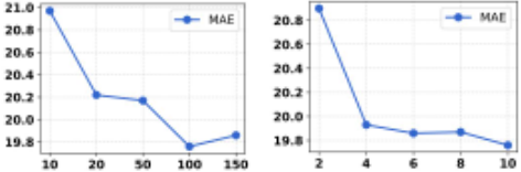
Figure 4: Sensitivity analysis of parameter K and M on PEMS07 dataset.
It is evident that setting K or M too low results in a sharp decline in performance. This is because an insufficient number of subgraphs or nodes per subgraph leads to inadequate extraction of spatio-temporal features, causing the model to underfit and fail to achieve the same performance as the original model. When the product of K and M approaches or exceeds N, the performance of DDGCRN-SGL matches that of DDGCRN, while requiring significantly less memory. Therefore, properly configuring K and M is crucial for balancing memory efficiency and maintaining performance.
4.4 Subgraph Visualization (Q4)
In this section, we visualize the subgraphs generated by DDGCRN-SGL during prediction on the test set to analyze the feature similarity among subgraph nodes and the distribution of overlapping nodes across subgraphs. Figure 5 presents the visualization results of subgraph features after dimensionality reduction using the T-SNE algorithm [Van der Maaten and Hinton, 2008].
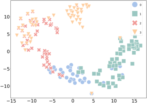
The results show that the nodes in each subgraph exhibit clustering behavior, indicating a high degree of similarity among nodes selected based on their feature similarity. Additionally, the visualization reveals overlapping or closely located nodes across different subgraphs, demonstrating that some nodes are shared among multiple subgraphs. This overlap further validates the necessity of the SGFAM module to address potential redundancies in aggregated node feature.
5 Conclusion
In this paper, we propose a plug-and-play SubGraph Learning method to reduce the memory overhead of spatio-temporal graph models. Specifically, we introduce a SubGraph Partition Module that dynamically partitions the original spatiotemporal graph into smaller subgraphs for extracting spatial features, significantly reducing memory overhead. To address the issue of redundant node feature caused by nodes appearing in multiple subgraphs, we design an SubGraph Feature Aggregation Module that performs average aggregation on the multiple features obtained by nodes. We conduct a comprehensive evaluation of this method on traffic network datasets of various scales, and the results demonstrate that it can significantly reduce GPU consumption without compromising model performance, providing a practical solution for deploying spatio-temporal models in real-world scenarios.
Acknowledgments
This work was supported in part by the "Pioneer" and "Leading Goose" R&D Program of Zhejiang under Grant 2024C01214, in part by the National Natural Science Foundation of China under Grant 62072409 and 62476247, and Zhejiang Supcon Information Co., Ltd. KYY-HX-20230833.
@inproceedings{ijcai2025p386,
  title     = {Let’s Group: A Plug-and-Play SubGraph Learning Method for Memory-Efficient Spatio-Temporal Graph Modeling},
  author    = {Weng, Wenchao and Jiang, Hanyu and Wu, Mei and Han, Xiao and Gao, Haidong and Shen, Guojiang and Kong, Xiangjie},
  booktitle = {Proceedings of the Thirty-Fourth International Joint Conference on
               Artificial Intelligence, {IJCAI-25}},
  publisher = {International Joint Conferences on Artificial Intelligence Organization},
  editor    = {James Kwok},
  pages     = {3471--3479},
  year      = {2025},
  month     = {8},
  note      = {Main Track},
  doi       = {10.24963/ijcai.2025/386},
  url       = {https://doi.org/10.24963/ijcai.2025/386},
}
TY - CPAPER TI - Let’s Group: A Plug-and-Play SubGraph Learning Method for Memory-Efficient Spatio-Temporal Graph Modeling AU - Weng, Wenchao AU - Jiang, Hanyu AU - Wu, Mei AU - Han, Xiao AU - Gao, Haidong AU - Shen, Guojiang AU - Kong, Xiangjie T2 - Proceedings of the Thirty-Fourth International Joint Conference on Artificial Intelligence, IJCAI-25 PB - International Joint Conferences on Artificial Intelligence Organization PY - 2025 SP - 3471 EP - 3479 DO - 10.24963/ijcai.2025/386 UR - https://doi.org/10.24963/ijcai.2025/386 ER -Copied
Machine-readable versions of this paper, for tools and AI agents:





