
CAN-ST: Clustering Adaptive Normalization for Spatio-temporal OOD Learning
Proceedings of the Thirty-Fourth International Joint Conference on Artificial Intelligence. Main Track. Pages 3543-3551.
https://doi.org/10.24963/ijcai.2025/394
Keywords
- Data Mining: DM: Mining data streams
- Data Mining: DM: Applications
- Data Mining: DM: Mining spatial and/or temporal data
Abstract
Spatio-temporal data mining is crucial for decision-making and planning in diverse domains. However, in real-world scenarios, training and testing data are often not independent or identically distributed due to rapid changes in data distributions over time and space, resulting in spatio-temporal out-of-distribution (OOD) challenges. This non-stationarity complicates accurate predictions and has motivated research efforts focused on mitigating non-stationarity through normalization operations. Existing methods, nonetheless, often address individual time series in isolation, neglecting correlations across series, which limits their capacity to handle complex spatio-temporal dynamics and results in suboptimal solutions. To overcome these challenges, we propose Clustering Adaptive Normalization (CAN-ST), a general and model-agnostic method that mitigates non-stationarity by capturing both localized distributional changes and shared patterns across nodes via adaptive clustering and a parameter register. As a plugin, CAN-ST can be easily integrated into various spatio-temporal prediction models. Extensive experiments on multiple datasets with diverse forecasting models demonstrate that CAN-ST consistently improves performance by over 20% on average and outperforms state-of-the-art normalization methods.
- [An et al., 2024] Yang An, Zhibin Li, Wei Liu, Haoliang Sun, Meng Chen, Wenpeng Lu, and Yongshun Gong. Spatio-temporal graph normalizing flow for probabilistic traffic prediction. In Proceedings of the 33rd ACM Inter- national Conference on Information and Knowledge Man- agement, page 45-55, New York, NY, USA, 2024. Asso- ciation for Computing Machinery.
- [Angryk et al., 2020] Rafal A Angryk, Petrus C Martens, Berkay Aydin, Dustin Kempton, Sushant S Mahajan, Sunitha Basodi, Azim Ahmadzadeh, Xumin Cai, Soukaina Filali Boubrahimi, Shah Muhammad Hamdi, et al. Multi- variate time series dataset for space weather data analytics. Scientific data, 7(1):227, 2020.
- [Bai et al., 2020] Lei Bai, Lina Yao, Can Li, Xianzhi Wang, and Can Wang. Adaptive graph convolutional recurrent network for traffic forecasting. Advances in neural infor- mation processing systems, 33:17804-17815, 2020.
- [Dai and Van Gool, 2018] Dengxin Dai and Luc Van Gool. Dark model adaptation: Semantic image segmentation from daytime to nighttime. In 2018 21st International Conference on Intelligent Transportation Systems (ITSC), pages 3819-3824. IEEE, 2018.
- [Dai et al., 2024] Tao Dai, Beiliang Wu, Peiyuan Liu, Naiqi Li, Xue Yuerong, Shu-Tao Xia, and Zexuan Zhu. Ddn: Dual-domain dynamic normalization for non-stationary time series forecasting. In The Thirty-eighth Annual Con- ference on Neural Information Processing Systems, 2024.
- [Deng et al., 2021] Jinliang Deng, Xiusi Chen, Renhe Jiang, Xuan Song, and Ivor W Tsang. St-norm: Spatial and tem- poral normalization for multi-variate time series forecast- ing. In Proceedings of the 27th ACM SIGKDD conference on knowledge discovery & data mining, pages 269-278, 2021.
- [Deng et al., 2022] Jinliang Deng, Xiusi Chen, Renhe Jiang, Xuan Song, and Ivor W Tsang. A multi-view multi-task learning framework for multi-variate time series forecast- ing. IEEE Transactions on Knowledge and Data Engineer- ing, 35(8):7665-7680, 2022.
- [Deng et al., 2023] Pan Deng, Yu Zhao, Junting Liu, Xi- aofeng Jia, and Mulan Wang. Spatio-temporal neural structural causal models for bike flow prediction. In Pro- ceedings of the AAAI conference on artificial intelligence, volume 37, pages 4242-4249, 2023.
- [Deng et al., 2024a] Jinliang Deng, Xiusi Chen, Renhe Jiang, Du Yin, Yi Yang, Xuan Song, and Ivor W Tsang. Disentangling structured components: Towards adaptive, interpretable and scalable time series forecasting. IEEE Transactions on Knowledge and Data Engineering, 2024.
- [Deng et al., 2024b] Jinliang Deng, Feiyang Ye, Du Yin, Xuan Song, Ivor Tsang, and Hui Xiong. Parsimony or capability? decomposition delivers both in long-term time series forecasting. Advances in Neural Information Pro- cessing Systems, 37:66687-66712, 2024.
- [Dong et al., 2024] Zheng Dong, Renhe Jiang, Haotian Gao, Hangchen Liu, Jinliang Deng, Qingsong Wen, and Xuan Song. Heterogeneity-informed meta-parameter learning for spatiotemporal time series forecasting. In Proceedings of the 30th ACM SIGKDD conference on knowledge dis- covery and data mining, pages 631-641, 2024.
- [Du et al., 2021] Yuntao Du, Jindong Wang, Wenjie Feng, Sinno Pan, Tao Qin, Renjun Xu, and Chongjun Wang. Adarnn: Adaptive learning and forecasting of time se- ries. In Proceedings of the 30th ACM international con- ference on information & knowledge management, pages 402-411, 2021.
- [Fan et al., 2023] Wei Fan, Pengyang Wang, Dongkun Wang, Dongjie Wang, Yuanchun Zhou, and Yanjie Fu. Dish-ts: a general paradigm for alleviating distribution shift in time series forecasting. In Proceedings of the AAAI conference on artificial intelligence, volume 37, pages 7522-7529, 2023.
- [Gong et al., 2024] Yongshun Gong, Tiantian He, Meng Chen, Bin Wang, Liqiang Nie, and Yilong Yin. Spatio- temporal enhanced contrastive and contextual learning for weather forecasting. IEEE Transactions on Knowledge and Data Engineering, 2024.
- [He et al., 2016] Kaiming He, Xiangyu Zhang, Shaoqing Ren, and Jian Sun. Deep residual learning for image recog- nition. In Proceedings of the IEEE conference on computer vision and pattern recognition, pages 770-778, 2016.
- [Jiang et al., 2021] Renhe Jiang, Du Yin, Zhaonan Wang, Yizhuo Wang, Jiewen Deng, Hangchen Liu, Zekun Cai, Jinliang Deng, Xuan Song, and Ryosuke Shibasaki. Dl- traff: Survey and benchmark of deep learning models for urban traffic prediction. In Proceedings of the 30th ACM international conference on information & knowl- edge management, pages 4515-4525, 2021.
- [Jin et al., 2023] Yilun Jin, Kai Chen, and Qiang Yang. Transferable graph structure learning for graph-based traf- fic forecasting across cities. In Proceedings of the 29th ACM SIGKDD Conference on Knowledge Discovery and Data Mining, pages 1032-1043, 2023.
- [Kim et al., 2021] Taesung Kim, Jinhee Kim, Yunwon Tae, Cheonbok Park, Jang-Ho Choi, and Jaegul Choo. Re- versible instance normalization for accurate time-series forecasting against distribution shift. In International Con- ference on Learning Representations, 2021.
- [Kingma, 2014] Diederik P Kingma. Adam: A method for stochastic optimization. arXiv preprint arXiv:1412.6980, 2014.
- [Lai et al., 2018] Guokun Lai, Wei-Cheng Chang, Yiming Yang, and Hanxiao Liu. Modeling long-and short-term temporal patterns with deep neural networks. In The 41st international ACM SIGIR conference on research & devel- opment in information retrieval, pages 95-104, 2018.
- [Li et al., 2024] Xiaoyu Li, Yongshun Gong, Wei Liu, Yi- long Yin, Yu Zheng, and Liqiang Nie. Dual-track spatio- temporal learning for urban flow prediction with adaptive normalization. Artificial Intelligence, 328:104065, 2024.
- [Liu et al., 2023] Hangchen Liu, Zheng Dong, Renhe Jiang, Jiewen Deng, Jinliang Deng, Quanjun Chen, and Xuan Song. Spatio-temporal adaptive embedding makes vanilla transformer sota for traffic forecasting. In Proceedings of the 32nd ACM international conference on information and knowledge management, pages 4125-4129, 2023.
- [Liu et al., 2024] Zhiding Liu, Mingyue Cheng, Zhi Li, Zhenya Huang, Qi Liu, Yanhu Xie, and Enhong Chen. Adaptive normalization for non-stationary time series forecasting: A temporal slice perspective. Advances in Neural Information Processing Systems, 36, 2024.
- [Ogasawara et al., 2010] Eduardo Ogasawara, Leonardo C Martinez, Daniel De Oliveira, Geraldo Zimbrão, Gisele L Pappa, and Marta Mattoso. Adaptive normalization: A novel data normalization approach for non-stationary time series. In The 2010 International Joint Conference on Neu- ral Networks (IJCNN), pages 1-8. IEEE, 2010.
- [Passalis et al., 2019] Nikolaos Passalis, Anastasios Tefas, Juho Kanniainen, Moncef Gabbouj, and Alexandros Iosi- fidis. Deep adaptive input normalization for time series forecasting. IEEE transactions on neural networks and learning systems, 31(9):3760-3765, 2019.
- [Qu et al., 2022] Hao Qu, Yongshun Gong, Meng Chen, Junbo Zhang, Yu Zheng, and Yilong Yin. Forecasting fine- grained urban flows via spatio-temporal contrastive self- supervision. IEEE Transactions on Knowledge and Data Engineering, 35(8):8008-8023, 2022.
- [Wang et al., 2024a] Binwu Wang, Jiaming Ma, Pengkun Wang, Xu Wang, Yudong Zhang, Zhengyang Zhou, and Yang Wang. Stone: A spatio-temporal ood learning frame- work kills both spatial and temporal shifts. In Proceedings of the 30th ACM SIGKDD Conference on Knowledge Dis- covery and Data Mining, pages 2948-2959, 2024.
- [Wang et al., 2024b] Hongjun Wang, Jiyuan Chen, Tong Pan, Zheng Dong, Lingyu Zhang, Renhe Jiang, and Xuan Song. Evaluating the generalization ability of spa- tiotemporal model in urban scenario. arXiv preprint arXiv:2410.04740, 2024.
- [Wu et al., 2019] Zonghan Wu, Shirui Pan, Guodong Long, Jing Jiang, and Chengqi Zhang. Graph wavenet for deep spatial-temporal graph modeling. arXiv preprint arXiv:1906.00121, 2019. IJCAI
- [Xia et al., 2024] Yutong Xia, Yuxuan Liang, Haomin Wen, Xu Liu, Kun Wang, Zhengyang Zhou, and Roger Zimmer- mann. Deciphering spatio-temporal graph forecasting: A causal lens and treatment. Advances in Neural Information Processing Systems, 36, 2024.
- [Yao et al., 2022] Huaxiu Yao, Caroline Choi, Bochuan Cao, Yoonho Lee, Pang Wei W Koh, and Chelsea Finn. Wild- time: A benchmark of in-the-wild distribution shift over time. Advances in Neural Information Processing Systems, 35:10309-10324, 2022.
- [Ye et al., 2024] Weiwei Ye, Songgaojun Deng, Qiaosha Zou, and Ning Gui. Frequency adaptive normalization for non-stationary time series forecasting. arXiv preprint arXiv:2409.20371, 2024.
- [Yu et al., 2017] Bing Yu, Haoteng Yin, and Zhanxing Zhu. Spatio-temporal graph convolutional networks: A deep learning framework for traffic forecasting. arXiv preprint arXiv:1709.04875, 2017. IJCAI
- [Zhou et al., 2023] Zhengyang Zhou, Qihe Huang, Kuo Yang, Kun Wang, Xu Wang, Yudong Zhang, Yuxuan Liang, and Yang Wang. Maintaining the status quo: Cap- turing invariant relations for ood spatiotemporal learning. In Proceedings of the 29th ACM SIGKDD Conference on Knowledge Discovery and Data Mining, pages 3603- 3614, 2023.
References were extracted automatically from the PDF and may contain errors.
Full text extracted automatically from the PDF; figures, tables and equations may differ. The PDF is the version of record.
1 Introduction
The rise of sensor networks has led to the widespread collection of spatio-temporal time series in urban environments. As these datasets expand rapidly, accurate spatio-temporal time series forecasting becomes increasingly crucial for various real-world applications, including transportation [Jiang et al., 2021; Jin et al., 2023], weather [Angryk et al., 2020; Gong et al., 2024], and economics [Lai et al., 2018; Dong et al., 2024]. Given the significance and urgency of urban spatio-temporal prediction, recent advancements in deep learning techniques [Li et al., 2024; Qu et al., 2022; An et al., 2024; Deng et al., 2024a; Deng et al., 2022; Deng et al., 2024b] have accelerated research in this domain.
∗Corresponding author.
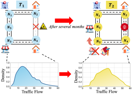
However, accurately predicting spatio-temporal patterns remains a challenge due to the rapid evolution of distributions over time, which results in spatio-temporal out-ofdistribution (OOD) scenarios [Liu et al., 2024]. One such example is illustrated in Figure 1, showing the dynamic evolution of urban areas. Several months ago during T1, subway construction disrupted the road between N2 and N4, altering spatial dependencies by weakening the N2-N4 correlation and strengthening the N2-N1 correlation. These changes reverted after the project was completed during T2. Additionally, the relocation of the entertainment mall at N3 to N5, expansion of the N2-N4 road for the subway station, and construction of a new residential building at N3 led to further shifts in spatial relations.
These changes altered the spatio-temporal joint distribution, rendering previous deep learning models ineffective. A decade ago, research showed that machine learning systems could fail significantly when evaluated on data outside the domain of their training examples, mainly due to their dependence on the training distribution [Dai and Van Gool, 2018; Wang et al., 2024b]. To alleviate the impact of distribution shifts, normalization methods have been proposed as a viable solution [Passalis et al., 2019; Liu et al., 2024]. These methods aim to remove non-stationary factors, infer output statistics from input statistics, and estimate the output distribution via de-normalization. However, these methods learn statistics evolution patterns for each location time series independently, overlooking potential shared patterns across spatial dimensions. As a result, when correlations between spatial nodes change, suboptimal solutions can arise.
For instance, in urban traffic flow prediction, changes at specific spatio-temporal nodes can lead to significant shifts in distribution patterns. As shown in Figure 1, the demolition of the entertainment mall at N3 and its replacement with a residential area during T1 caused a dramatic shift in observed patterns. Previous methods, which focused solely on individual locations, experienced notable performance degradation at this node during T2. In fact, the behavior at N3 during T2 could be inferred from data at other nodes, such as N2 and N4 during T1, as these locations exhibit similar trends to residential areas. In practice, this provided valuable insights, revealing shared patterns critical for understanding dynamics in spatio-temporal OOD learning.
This observation suggests the use of clustering to extract representative spatio-temporal patterns. When distribution shifts occur at a specific spatio-temporal node, these clusterlevel patterns can be leveraged to infer the new distribution, mitigating the impact of such changes. Motivated by this, we propose Clustering Adaptive Normalization (CAN-ST), a model-agnostic framework for spatio-temporal OOD learning. CAN-ST operates in three steps: (1) it normalizes input data using statistics to remove non-stationary factors, ensuring more reliable predictions; (2) it applies adaptive clustering to group spatio-temporal nodes with similar patterns, facilitating the extraction of representative spatio-temporal semantics and reducing reliance on individual historical time series; (3) it uses a parameter register to capture distributional evolution patterns specific to each cluster, enabling flexible and accurate de-normalization and distribution transformations, even under severe spatio-temporal OOD conditions.
Unlike existing methods that focus on individual nodes or time series, CAN-ST captures both localized distributional changes at each node and shared distributional evolution patterns among nodes within the same cluster. By integrating these features, CAN-ST ensures robust normalization and denormalization in spatio-temporal OOD scenarios. Extensive experiments conducted on widely used datasets demonstrate that CAN-ST significantly improves the performance of various mainstream prediction models, consistently outperforming state-of-the-art normalization approaches. In summary, our work makes the following key contributions:
- We introduce CAN-ST, a general normalization framework specifically designed for spatio-temporal OOD learning tasks. As a plugin, CAN-ST can be easily integrated into various spatio-temporal prediction models.
- We propose an adaptive spatio-temporal clustering
- method to capture shared distributional evolution patterns, along with a parameter register that ensures stable and flexible distribution transformations, even under spatio-temporal distribution shifts.
- We validate CAN-ST through extensive experiments on four real-world datasets. The results demonstrate that it consistently enhances predictive performance across mainstream models and surpasses state-of-the-art normalization methods, showcasing its effectiveness in tackling spatio-temporal OOD challenges.
2 RelatedWork
2.1 Spatio-temporal Out-of-Distribution Learning
Previous studies in spatio-temporal data mining have extensively explored out-of-distribution (OOD) challenges [Wang et al., 2024a; Du et al., 2021; Yao et al., 2022; Deng et al., 2023], laying the groundwork for understanding distributional shifts in real-world applications. Recent focus has shifted to OOD issues in spatio-temporal urban prediction, where urbanization and evolving mobility patterns introduce significant temporal and spatial discrepancies. Infrastructure changes, seasonal variations, and unforeseen events further exacerbate non-stationarity in urban data. Recent works [Xia et al., 2024; Zhou et al., 2023], address OOD scenarios using causal inference within spatio-temporal frameworks. Xia [2024] proposed a hybrid approach combining disentanglement blocks for backdoor adjustment and frontdoor adjustment with edge-level convolution. Zhou [2023] reformulated invariant learning to identify stable parameters robust under varying distributions. These methods highlight the potential of causal inference to mitigate OOD effects.
However, causality-based methods often require complex training, significant computational resources, and expertise, limiting scalability and real-time use. CAN-ST offers a practical and model-agnostic alternative. By tackling OOD challenges through a lightweight framework, CAN-ST balances computational efficiency with predictive accuracy, making it ideal for dynamic, non-stationary environments.
2.2 NormalizationMethods for Non-stationary Time Series Forecasting
Approaches to normalization have been devised to address the challenges posed by non-stationarity. To account for instance-specific variations, [Ogasawara et al., 2010] propose leveraging normalization techniques that rely on local characteristics rather than global statistics. Passalis [2019] advance this instance-wise normalization framework by introducing an adaptive and learnable approach. While these methods effectively eliminate non-stationary elements from inputs, predicting non-stationary time series in the outputs remains a significant challenge.
To address this, reversible instance normalization [Kim et al., 2021] was introduced, allowing the removed nonstationary components to be reintroduced for output reconstruction. However, it presumes consistent trends between inputs and outputs. Kim [2021] further refine this idea through RevIN, focusing on evolving trends within input sequences.
Recent studies [Fan et al., 2023; Ogasawara et al., 2010] delve into trend modeling at finer granularities, such as at the segment level. Additionally, Ye [2024] and Dai [2024] extended normalization using Fourier Transform to capture frequency-domain information.
These works focus on independent time series, ignoring spatio-temporal dependencies. In contrast, CAN-ST employs adaptive clustering to capture shared patterns and a parameter register to dynamically model local and global relationships.
3 ProblemDefinition
Let G = (V,E,A) represent a spatial network, where V and E denote the sets of vertices and edges, respectively. The adjacency matrix of G is denoted as A. Furthermore, we define the graph signal matrix xt ∈ RN×D for G, where D represents the feature dimension, N = |V | is the number of vertices, and xt represents the observations of G at time step t. Overall, the goal of spatio-temporal tasks is to learn a multistep prediction function f based on historical observations:
where T is the input length of past time step observations, and τ is the number of future steps we aim to predict.
Unlike traditional spatio-temporal learning tasks, spatiotemporal OOD learning allows the graph relationships to differ between training and testing phases and to evolve over time during training. Specifically, following the setup of previous works, we assume that the graph GTest , representing spatial relationships, and the spatio-temporal distribution pTest (X) in the test set differ from those in the training set, such that:
4 Methodology
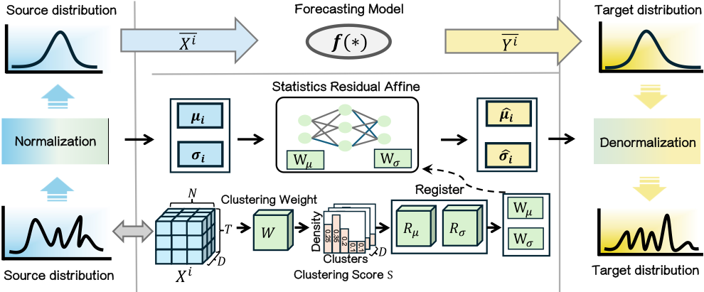
We propose a general, model-agnostic normalization framework for spatio-temporal OOD learning, termed Clustering Adaptive Normalization (CAN-ST), to address the aforementioned spatio-temporal distribution shift challenges. In this section, we provide a detailed explanation of the framework of CAN-ST and illustrate how it handles data affected by spatio-temporal distribution shifts. The whole framework CAN-ST be referred to in Figure 2.
4.1 Normalization
Given a spatio-temporal input denoted as Xi ∈ RT×N×D, which represents { xt-T , . . . , xt-1 }, CAN-ST normalizes the input to remove the non-stationary factors. Specifically, we normalize the input data Xi using its instance-specific mean and standard deviation, which is widely accepted as instance normalization [Kim et al., 2021]. The mean and standard deviation are computed for every spatio-temporal instance:
where ϵ is a small positive constant, typically set to 1×10⁻⁵ . Finally, the transformed ¯ Xi , with non-stationary factors removed, is used as the new input for the prediction model.
4.2 Adaptive Spatio-temporal Clustering
Unlike existing methods, which normalize and de-normalize only the time series of individual spatial nodes, CAN-ST addresses a natural challenge: how to estimate future evolution distributions without solely relying on historical time series in the presence of spatio-temporal distribution shifts?
In scenarios where such shifts occur, using the mean and variance of a single historical time series for de-normalization can lead to significant performance degradation, as the output statistics deviate from µi and σi. Additionally, for nodes introducing new spatio-temporal relationships (such as N3 at future temporal node in Figure 1), sharp changes in the spatiotemporal distribution create an urgent need for interactions with nodes that exhibit similar trends. To address these issues, it is essential to extract shared knowledge from similar spatio-temporal nodes as a reserve. During distribution shifts, the model can bypass sole reliance on the historical data of individual nodes for de-normalization by leveraging shared knowledge from all nodes. This shared knowledge is used to infer the required statistical properties for de-normalization, enabling a more robust transformation.
Motivated by this, CAN-ST clusters all spatio-temporal nodes to identify representative spatio-temporal patterns within the dataset. First, CAN-ST performs adaptive spatiotemporal clustering based on the input data. Unlike tasks in NLP and CV, where features generally correspond to similar types of information, each feature in urban spatio-temporal computing often conveys distinct meanings, such as vehicle speed and traffic volume. Therefore, we model each feature separately, as outlined below:
where W ∈ RD×TN×C is the clustering matrix. ˜ Xi ∈ RD×TN is the reshaping of Xi . C is the predefined number of spatio-temporal clusters. Each row of S[d, :] represents the probability of the spatio-temporal sample belonging to each cluster for feature d.
4.3 Statistics Residual Affine &Denormalization
Then, we performs match-based de-normalization according to the clustering results. To achieve more accurate denormalization, CAN-ST learns to infer the statistics of output.
To leverage the patterns of typical spatio-temporal clusters and eliminate reliance on the historical sequences of individual nodes, CAN-ST is equipped with transformation parameter registers. These registers store the statistics transformation patterns from input's distribution space to output's of each cluster. For given spatio-temporal nodes, the register is matched based on there clustering scores, producing affine coefficients that integrate global spatio-temporal dependencies. We assigns separate transformation parameter registers for the mean and variance, which are learned end-to-end alongside the prediction model. These registers are randomly initialized as Rµ ∈ RD×C×C′ and Rσ ∈ RD×C×C′ . Next, we match the spatio-temporal nodes with the parameter registers based on the clustering results to obtain transformation coefficients:
where W1 ∈ RC′×1 and W2 ∈ RC′×1 are learnable pooling weights used to reduce the dimension from C ′ to 1. Then Wµ ∈ RD×1 and Wσ ∈ RD×1 are used to infer the statistics of the output. We incorporate the residual learning technique [He et al., 2016] into our method, enabling the module to learn the difference between the statistics of the future output and the input, rather than directly predicting the exact value. This approach reduces the difficulty of mean modeling by leveraging prior knowledge of future trends:
where ⊙ denotes element-wise multiplication. While predicting the statistics, CAN-ST feeds the normalized spatiotemporal data into the prediction model f(∗), which generates the internal output ¯ Y . Finally, CAN-ST applies denormalization to the output from the prediction model f(∗), inferring the distribution of output to produce accurate predictions:
5 Experiment
In this section, we conduct sufficient experiments within a widely used benchmark dataset compared to state-of-the-art methods to evidence the effectiveness of our proposed CANST framework.
5.1 Experimental Setup
All experiments followed strict fairness protocols in a benchmark [Wang et al., 2024b].
Datasets: We conduct our experiments on four real-world datasets: BikeCHI 1 , TaxiCHI 2 , PEMS08 3 and SpeedNYC 4 . The details about these datasets are listed in the Table 1. We adhere to the in-distribution and out-of-distribution testing protocols outlined in to rigorously evaluate model performance. Specifically, models are trained on data from year A and subsequently evaluated on datasets from both year A (in-distribution) and year A + 1 (out-of-distribution), which has been proven to be reasonable [Wang et al., 2024b]. It should be noted that using data from year A for testing corresponds to the conventional experimental setup in spatiotemporal learning. We adopted the data partitioning strategy established in prior work [Jiang et al., 2021], which chronologically divides the data into training, validation, and testing subsets with a 6:2:2 ratio [Wang et al., 2024b].
1 https://www.divvybikes.com/system-Data
2 https://data.cityofchicago.org/
3 https://pems.dot.ca.gov/
4 https://www.nyc.gov/html/dot/html/motorist/atis.shtml
| Dataset | Application | City/State | Train Year | Train Span | Test Year | Test Span | Nodes | Interval |
|---|---|---|---|---|---|---|---|---|
| BikeCHI | Bike-sharing | Chicago | 2019 | 01.01 - 10.19 | 2019/2020 | 10.20 - 12.31 | 609 | 60 mins |
| TaxiCHI | Ride-sharing | Chicago | 2013 | 01.01 - 10.19 | 2013/2014 | 10.20 - 12.31 | 77 | 60 mins |
| SpeedNYC | Vehicle Speed | NYC | 2019 | 03.01 - 05.12 | 2019/2020 | 05.13 - 05.31 | 139 | 5 mins |
| PEMS08 | Traffic Flow | California | 2016 | 07.01 - 08.18 | 2017/2018 | 08.19 - 08.31 | 170 | 5 mins |
| Model | TaxiCHI 1 hour | TaxiCHI 3 hours | BikeCHI 1 hour | BikeCHI 3 hours | PEMS08 5 mins | PEMS08 15 mins | SpeedNYC 5 mins | SpeedNYC 15 mins | ||||||||
|---|---|---|---|---|---|---|---|---|---|---|---|---|---|---|---|---|
| RMSE | MAE | RMSE | MAE | RMSE | MAE | RMSE | MAE | RMSE | MAE | RMSE | MAE | RMSE | MAE | RMSE | MAE | |
| STAEformer | 33.07 | 10.31 | 44.94 | 13.35 | 2.10 | 1.15 | 2.43 | 1.26 | 19.69 | 11.92 | 21.66 | 12.74 | 4.83 | 2.78 | 7.00 | 4.21 |
| +CAN-ST | 24.28 | 8.24 | 34.83 | 10.73 | 2.06 | 1.14 | 2.27 | 1.22 | 19.54 | 11.82 | 21.56 | 12.67 | 4.90 | 2.89 | 6.85 | 4.15 |
| ∆ | 26.58%20.08%22.50%19.63% | 1.90% | 0.87% | 6.58% | 3.17% | 0.76% | 0.84% | 0.46% | 0.55% | -1.45%-3.96% | 2.14% | 1.43% | ||||
| STGCN | 38.54 | 11.89 | 47.84 | 14.23 | 2.19 | 1.21 | 2.44 | 1.27 | 22.66 | 15.17 | 24.30 | 15.97 | 5.51 | 3.45 | 7.04 | 4.44 |
| +CAN-ST | 27.32 | 9.51 | 35.93 | 11.44 | 2.08 | 1.19 | 2.28 | 1.26 | 21.34 | 14.14 | 23.27 | 15.22 | 5.23 | 3.13 | 6.96 | 4.29 |
| ∆ | 29.11%20.02%24.90%19.61% | 5.02% | 1.65% | 6.56% | 0.79% | 5.83% | 6.79% | 4.24% | 4.70% | 5.08% | 9.28% | 1.14% | 3.38% | |||
| GWNET | 29.19 | 9.30 | 44.39 | 13.78 | 2.78 | 1.31 | 2.78 | 1.24 | 19.91 | 12.60 | 22.24 | 13.63 | 4.85 | 2.77 | 6.82 | 4.20 |
| +CAN-ST | 22.32 | 8.36 | 34.95 | 11.25 | 2.09 | 1.16 | 2.32 | 1.21 | 19.67 | 12.49 | 21.89 | 13.57 | 4.81 | 2.76 | 6.86 | 4.19 |
| ∆ | 23.54%10.11%21.27%18.36%24.82%11.45%16.55%0.83% | 1.21% | 0.87% | 1.57% | 0.44% | 0.82% | 0.36% | -0.59% | 0.24% | |||||||
| AGCRN | 33.83 | 9.94 | 46.06 | 13.85 | 2.06 | 1.14 | 2.32 | 1.23 | 20.91 | 13.49 | 22.61 | 14.33 | 5.41 | 3.17 | 7.13 | 5.41 |
| +CAN-ST | 24.20 | 8.35 | 34.55 | 10.85 | 2.06 | 1.14 | 2.30 | 1.22 | 20.43 | 13.14 | 22.32 | 14.17 | 5.04 | 2.98 | 6.89 | 4.32 |
| ∆ | 28.47%16.00%24.99%21.66% | 0.00% | 0.00% | 0.86% | 0.81% | 2.30% | 2.59% | 1.28% | 1.12% | 6.84% | 5.99% | 3.37% | 25.23% | |||
Backbone models: CAN-ST is a model-agnostic framework applicable to any spatio-temporal forecasting model f(∗). To demonstrate the effectiveness of the framework, we select several mainstream models based on different architectures and evaluate their performance under both in-distribution and out-of-distribution conditions: the dilated convolution and graph convolution based Graph WaveNet [Wu et al., 2019], the Transformer-based STAEformer [Liu et al., 2023], the recurrent neural network and graph convolution based AGCRN [Bai et al., 2020], and the temporal convolution and graph convolution based STGCN [Yu et al., 2017]. We follow the implementation and settings provided in the official code of the spatio-temporal OOD learning benchmark [Wang et al., 2024b].
Experiments details: We use ADAM [Kingma, 2014] as the default optimizer across all the experiments and report the root mean squared error (RMSE) and mean absolute error (MAE) as the evaluation metrics.
5.2 Main Results
We present the spatio-temporal prediction results in Table 2 and Table 3. For the TaxiCHI and BikeCHI datasets, the prediction horizons are set to {1 hour, 3 hours}, while for other datasets, the horizons are {5 minutes, 15 minutes}. Regarding the input sequence length, we follow standard protocols, fixing the input window length to 12 hours for the TaxiCHI and BikeCHI datasets and 1 hour for the remaining datasets. From these results, we derive several key observations as follows:
- CAN-ST consistently delivers substantial performance gains across multiple datasets and testing scenarios. Both RMSE and MAE metrics show that models equipped with CAN-ST outperform their baseline counterparts in most cases. This demonstrates the adaptability of CAN-ST in varying testing environments, including both In-Distribution (IN) and Out-of-Distribution (OUT) settings.
- CAN-ST effectively enhances both Transformer-based models (e.g., STAEformer) and GCN-based models (e.g., STGCN, GWNET, and AGCRN). Specifically, CAN-ST achieves an average relative performance improvement of 22.32%, 22.24%, 19.33%, and 24.24% over STAEformer, STGCN, GWNET, and AGCRN, respectively.
- Under out-of-distribution testing, CAN-augmented models show substantial improvements. For instance, integrating CAN-ST reduces STAEformer's RMSE on TaxiCHI by 46.5% (1-hour: 63.08→31.50; 3-hour: 83.38→44.63). Consistent gains across other models highlight CAN's efficacy in adapting to distribution shifts.
- The observed performance gains are consistent across different baseline architectures, including STAEformer, STGCN, GWNET, and AGCRN. This underlines the generalizability and compatibility of CAN-ST as a plug-in module for spatio-temporal prediction tasks.
5.3 Comparison with Advanced Normalization Methods
In this section, we compare CAN-ST with state-of-the-art normalization methods, including SAN [Liu et al., 2024]
| Model | TaxiCHI 1 hour | TaxiCHI 3 hours | BikeCHI 1 hour | BikeCHI 3 hours | PEMS08 5 mins | PEMS08 15 mins | SpeedNYC 5 mins | SpeedNYC 15 mins | ||||||||
|---|---|---|---|---|---|---|---|---|---|---|---|---|---|---|---|---|
| RMSE | MAE | RMSE | MAE | RMSE | MAE | RMSE | MAE | RMSE | MAE | RMSE | MAE | RMSE | MAE | RMSE | MAE | |
| STAEformer | 63.08 | 16.15 | 83.38 | 22.01 | 3.59 | 1.88 | 4.10 | 2.06 | 29.49 | 19.75 | 37.76 | 25.04 | 6.57 | 3.82 | 8.34 | 5.09 |
| +CAN-ST | 31.50 | 10.12 | 44.63 | 13.64 | 3.40 | 1.85 | 4.03 | 2.05 | 27.62 | 17.86 | 35.26 | 22.50 | 6.70 | 3.85 | 8.18 | 4.94 |
| ∆ | 50.06%37.34%46.47%38.03% | 5.29% | 1.60% | 1.71% | 0.49% | 6.34% | 9.57% | 6.62% | 10.14% | -1.98%-0.79% | 1.92% | 2.95% | ||||
| STGCN | 73.85 | 20.34 | 86.47 | 23.57 | 3.72 | 1.97 | 4.10 | 2.10 | 93.57 | 62.64 | 99.70 | 67.36 | 8.31 | 5.41 | 9.30 | 6.17 |
| +CAN-ST | 35.19 | 11.85 | 45.95 | 14.42 | 3.27 | 1.86 | 3.74 | 2.00 | 81.25 | 55.34 | 85.02 | 58.48 | 8.12 | 5.10 | 9.46 | 6.10 |
| ∆ | 52.35%41.74%46.86%38.82%12.10%5.58% | 8.78% | 4.76%13.17%11.65%14.72%13.18% | 2.29% | 5.73% | -1.72% | 1.13% | |||||||||
| GWNET | 48.69 | 13.21 | 76.17 | 21.03 | 3.18 | 1.75 | 3.58 | 1.95 | 24.60 | 15.91 | 30.89 | 19.61 | 6.14 | 3.42 | 7.42 | 4.53 |
| +CAN-ST | 26.63 | 9.48 | 43.47 | 13.67 | 3.01 | 1.74 | 3.56 | 1.93 | 23.99 | 15.55 | 29.76 | 18.94 | 6.27 | 3.37 | 7.27 | 4.21 |
| ∆ | 45.31%28.24%42.93%35.00% | 5.35% | 0.57% | 0.56% | 1.03% | 2.48% | 2.26% | 3.66% | 3.42% | -2.12% | 1.46% | 2.02% | 7.06% | |||
| AGCRN | 60.60 | 15.56 | 80.63 | 22.29 | 3.25 | 1.81 | 3.87 | 2.04 | 45.39 | 32.45 | 55.07 | 39.30 | 7.42 | 4.64 | 8.68 | 5.62 |
| +CAN-ST | 29.67 | 9.81 | 43.40 | 13.53 | 3.18 | 1.81 | 3.69 | 2.01 | 37.74 | 25.47 | 44.69 | 30.93 | 7.83 | 4.62 | 9.26 | 5.80 |
| ∆ | 51.04%36.95%46.17%39.30% | 2.15% | 0.00% | 4.65% | 1.47%16.85%21.51%18.85%21.30% | -5.53% | 0.43% | -6.68%-3.20% | ||||||||
and Dish-TS [Fan et al., 2023] for non-stationary time series forecasting, ST-Norm [Deng et al., 2021] for non-stationary spatio-temporal forecasting, and Z-score normalization. For the TaxiCHI and BikeCHI datasets, the prediction horizons are set to {1 hour, 2 hours, . . . , 12 hours}. Regarding the input sequence length, we follow the same experimental settings outlined in Section 5.2. We report the average results across all prediction horizons for STAEformer, STGCN, GWNET, and AGCRN, as well as the relative improvements in Table 4, revealing CAN-ST demonstrates superior performance compared to existing normalization methods across all evaluated scenarios and models. The experimental results validate the effectiveness of CAN-ST and highlight its key design advantages, which can be attributed to following primary factors:
(1) Unlike traditional normalization methods, such as ZScore, which apply static transformations based on fixed statistical metrics calculated from the entire dataset, CAN-ST introduces a dynamic mechanism that adapts to evolving distributional patterns. This adaptability ensures that the normalization process remains aligned with the underlying data distribution, effectively mitigating the impact of distribution shifts and enhancing the robustness and accuracy of downstream predictive models.
(2) Compared to SAN and DishST, which focus on single time series for the specific spatial node, CAN-ST provides a more comprehensive solution by simultaneously addressing localized and shared distributional changes through cluster spatio-temporal nodes. This holistic approach makes it more robust in diverse scenarios.
(3) STNorm's dependence on global statistics limits its effectiveness under spatio-temporal distribution shifts (e.g., emerging nodes or dynamic node behaviors). In contrast, CAN-ST dynamically clusters similar nodes and adapts transformation parameters, maintaining robust performance despite severe shifts.
| Methods | IN | OUT | ||||||
|---|---|---|---|---|---|---|---|---|
| BikeCHI | TaxiCHI | BikeCHI | TaxiCHI | |||||
| RMSE | MAE | RMSE | MAE | RMSE | MAE | RMSE | MAE | |
| Z-Score | 2.64 | 1.32 | 46.64 | 13.83 | 4.48 | 2.14 | 80.78 | 21.78 |
| STAEformer ST-Norm | 2.48 | 1.26 | 53.95 | 17.04 | 4.38 | 2.14 | 91.31 | 25.76 |
| SAN | 2.75 | 1.40 | 55.50 | 16.57 | 4.10 | 2.16 | 67.70 | 19.52 |
| DishST | 3.23 | 1.73 | 41.95 | 12.57 | 4.01 | 2.29 | 50.89 | 14.81 |
| CAN-ST | 2.35 | 1.25 | 38.87 | 11.70 | 3.88 | 2.05 | 49.22 | 14.68 |
| Z-Score | 2.64 | 1.34 | 49.71 | 14.74 | 4.32 | 2.15 | 87.83 | 23.94 |
| STGCN ST-Norm | 2.55 | 1.33 | 52.34 | 15.77 | 4.46 | 2.17 | 89.66 | 25.44 |
| SAN | 3.26 | 1.57 | 85.82 | 26.82 | 4.18 | 2.22 | 105.07 | 31.21 |
| DishST | 2.79 | 1.88 | 66.08 | 21.19 | 3.75 | 2.32 | 79.26 | 24.52 |
| CAN-ST | 2.45 | 1.31 | 39.73 | 12.22 | 3.69 | 2.00 | 50.42 | 15.41 |
| Z-Score | 2.51 | 1.29 | 48.57 | 14.96 | 3.99 | 2.04 | 76.51 | 20.97 |
| GWNET ST-Norm | 2.96 | 1.47 | 49.22 | 14.62 | 4.44 | 2.21 | 83.06 | 22.28 |
| SAN | 3.40 | 1.61 | 41.25 | 12.56 | 4.19 | 2.22 | 51.22 | 14.99 |
| DishST | 3.35 | 1.69 | 44.57 | 13.39 | 3.82 | 2.15 | 53.73 | 15.46 |
| CAN-ST | 2.43 | 1.28 | 39.26 | 12.34 | 3.68 | 2.01 | 49.37 | 14.97 |
| Z-Score | 2.47 | 1.27 | 51.95 | 15.35 | 3.99 | 2.08 | 90.20 | 24.93 |
| AGCRN ST-Norm | 2.54 | 1.28 | 133.83 | 30.85 | 4.06 | 2.15 | 178.02 | 41.14 |
| SAN | 3.37 | 1.62 | 59.50 | 18.36 | 4.15 | 2.21 | 74.28 | 22.00 |
| DishST | 3.38 | 1.70 | 50.32 | 16.37 | 4.67 | 2.34 | 58.52 | 18.71 |
| CAN-ST | 2.40 | 1.26 | 39.33 | 11.95 | 3.75 | 2.04 | 48.59 | 14.61 |
5.4 Investigation of Clustering Approaches
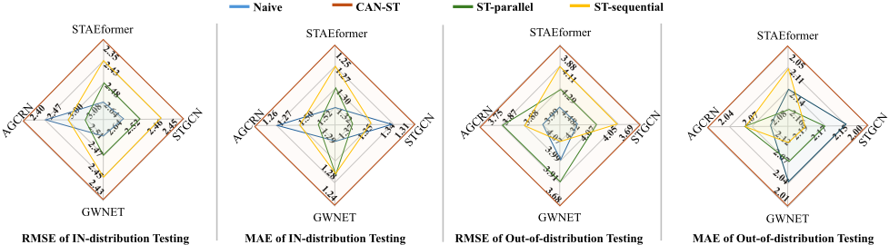
In this section, we investigate the impact of different clustering methods on experimental results. We examined three approaches ann presented the results in Figure 3.
- Naive: Do not utilize clustering approaches.
- CAN-ST: Our method clusters both temporal and spatial nodes of the input space simultaneously.
- ST-parallel: This approach clusters temporal and spatial nodes separately in parallel, matches them with the parameter register, and then fuses the results to obtain the affine coefficients.
- ST-sequential: This method clusters using the entire temporal sequence of spatial nodes, directly matching them with the parameter register to derive the affine coefficients.
CAN-ST consistently achieves the lowest RMSE and MAE by effectively modeling spatio-temporal patterns, outperforming other methods in both stable and shifting data distributions. While ST-sequential shows moderate robustness, and ST-parallel offers limited flexibility, both occasionally underperform baseline methods. In contrast, CAN-ST maintains robust superiority, demonstrating that simple parallel or sequential feature processing fails to capture complex spatiotemporal dynamics effectively.
5.5 Hyperparameters Analysis
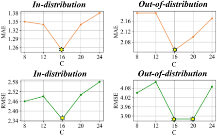
CAN-ST clusters spatio-temporal nodes into C classes based on their spatio-temporal distributions, where C is the size of Wc in Section 4.2. We analyze the influence of different C values on prediction accuracy in Figure 4. When C = 16, the model consistently achieves optimal performance. Although the RMSE under the Out-of-Distribution testing setting is minimized when C = 20, other metrics are not consistently optimal in this configuration. Consequently, it is evident that performance significantly outperforms other variants in most cases when using the most appropriate C, highlighting the effectiveness of clustering.
5.6 Discussion of Complexity and Runtime
We analyze the computational overhead of CAN-ST through theoretical complexity analysis and empirical runtime measurements. The framework introduces three main lightweight components: Normalization: Instance-wise statistics calculation (Eqs. 1-3) requires O(TND) operations; Adaptive Clustering: Feature-specific clustering (Eq. 6) has O(DTNC) complexity, where C (default 16) denotes cluster count. This scales linearly with T, N, and D; Parameter Register: Transformation coefficient derivation (Eqs. 7-8) involves O(DCC ′ ) operations. On TaxiCHI (N = 77, T = 12), CAN-ST adds only 0.59s/epoch to STAEformer's training time (16.24s vs. 16.83s), demonstrating efficient computation while improving OOD performance. Similar observations were made on other datasets and backbone models.
6 Conclusion
In this study, we propose CAN-ST, a model-agnostic framework for spatio-temporal OOD learning. Its threestep approach-normalization, adaptive clustering, and cluster-aware denormalization-effectively handles distribution shifts by jointly modeling local variations and global patterns. Experiments validate CAN-ST's superior performance over SOTA methods across diverse models and datasets.
Acknowledgments
This work was supported in part by the National Natural Science Foundation of China (62476154, 62202270), and Major Basic Research Project of Shandong Provincial Natural Science Foundation (ZR2024ZD03) and the Shandong Excellent Young Scientists Fund (Oversea) (2022HWYQ044), and the Taishan Scholar Project of Shandong Province (tsqn202306066), and Shandong University Qilu Young Scholars Program.
@inproceedings{ijcai2025p394,
  title     = {CAN-ST: Clustering Adaptive Normalization for Spatio-temporal OOD Learning},
  author    = {Yang, Min and An, Yang and Deng, Jinliang and Li, Xiaoyu and Xu, Bin and Zhong, Ji and Lu, Xiankai and Gong, Yongshun},
  booktitle = {Proceedings of the Thirty-Fourth International Joint Conference on
               Artificial Intelligence, {IJCAI-25}},
  publisher = {International Joint Conferences on Artificial Intelligence Organization},
  editor    = {James Kwok},
  pages     = {3543--3551},
  year      = {2025},
  month     = {8},
  note      = {Main Track},
  doi       = {10.24963/ijcai.2025/394},
  url       = {https://doi.org/10.24963/ijcai.2025/394},
}
TY - CPAPER TI - CAN-ST: Clustering Adaptive Normalization for Spatio-temporal OOD Learning AU - Yang, Min AU - An, Yang AU - Deng, Jinliang AU - Li, Xiaoyu AU - Xu, Bin AU - Zhong, Ji AU - Lu, Xiankai AU - Gong, Yongshun T2 - Proceedings of the Thirty-Fourth International Joint Conference on Artificial Intelligence, IJCAI-25 PB - International Joint Conferences on Artificial Intelligence Organization PY - 2025 SP - 3543 EP - 3551 DO - 10.24963/ijcai.2025/394 UR - https://doi.org/10.24963/ijcai.2025/394 ER -Copied
Machine-readable versions of this paper, for tools and AI agents:





