
A Centrality-based Graph Learning Framework
Proceedings of the Thirty-Fourth International Joint Conference on Artificial Intelligence. Main Track. Pages 3588-3596.
https://doi.org/10.24963/ijcai.2025/399
Keywords
- Data Mining: DM: Mining graphs
- Machine Learning: ML: Representation learning
Abstract
Graph Neural Networks (GNNs) have become powerful models for both node- and graph-level tasks. While node-level learning focuses on individual nodes and their local structures, graph-level learning encounters challenges in capturing the global properties of graphs. In this paper, we conduct a theoretical and experimental analysis of existing graph-level learning frameworks and find that these frameworks typically adopt a single-view perspective based solely on node degree, which limits their ability to capture comprehensive graph characteristics.
To address these issues, we propose a multi-view approach that leverages different types of centrality measures to capture diverse aspects of graph structure. We design an attention-based mechanism to adaptively integrate these multiple views, and use it as a readout function to perform weighted summation of node embeddings, termed as Adaptive Centrality Readout (ACRead). ACRead demonstrates enhanced flexibility and effectiveness when integrated with various GNN architectures, outperforming state-of-the-art readout methods, including KerRead and Set Transformer.
Additionally, this multi-view centrality approach can serve as a standalone graph-level learning framework without relying on GNNs, referred to as Adaptive Centrality-based Graph Learning (ACGL), which achieves competitive performance by effectively combining different centrality perspectives.
- [Balcilar et al., 2021] Muhammet Balcilar, Pierre Héroux, Benoit Gauzere, Pascal Vasseur, Sébastien Adam, and Paul Honeine. Breaking the limits of message passing graph neural networks. In International Conference on Machine Learning, pages 599-608. PMLR, 2021.
- [Buterez et al., 2022] David Buterez, Jon Paul Janet, Steven J Kiddle, Dino Oglic, and Pietro Liò. Graph neural networks with adaptive readouts. In NeurIPS, pages 19746-19758, 2022.
- [Chen et al., 2019] Ting Chen, Song Bian, and Yizhou Sun. Are powerful graph neural nets necessary? a dissection on graph classification. arXiv preprint arXiv:1905.04579, 2019.
- [Gao and Ji, 2019] Hongyang Gao and Shuiwang Ji. Graph u-nets. In ICML, pages 2083-2092, 2019.
- [Gao et al., 2020] Difei Gao, Ke Li, Ruiping Wang, Shiguang Shan, and Xilin Chen. Multi-modal graph neu- ral network for joint reasoning on vision and scene text. In Proceedings of the IEEE/CVF conference on computer vision and pattern recognition, pages 12746-12756, 2020.
- [Garg et al., 2020] Vikas Garg, Stefanie Jegelka, and Tommi Jaakkola. Generalization and representational limits of graph neural networks. In International Conference on Machine Learning, pages 3419-3430. PMLR, 2020.
- [Hamilton et al., 2017] Will Hamilton, Zhitao Ying, and Jure Leskovec. Inductive representation learning on large graphs. In NeurIPS, 2017.
- [Han et al., 2022] Kai Han, Yunhe Wang, Jianyuan Guo, Yehui Tang, and Enhua Wu. Vision gnn: An image is worth graph of nodes. Advances in neural information processing systems, 35:8291-8303, 2022.
- [Hu et al., 2020] Weihua Hu, Matthias Fey, Marinka Zitnik, Yuxiao Dong, Hongyu Ren, Bowen Liu, Michele Catasta, and Jure Leskovec. Open graph benchmark: Datasets for machine learning on graphs. Advances in neural informa- tion processing systems, 33:22118-22133, 2020.
- [Koh et al., 2024] Huan Yee Koh, Anh TN Nguyen, Shirui Pan, Lauren T May, and Geoffrey I Webb. Physicochemi- cal graph neural network for learning protein-ligand inter- action fingerprints from sequence data. Nature Machine Intelligence, pages 1-15, 2024.
- [Lee et al., 2021] Dongha Lee, Su Kim, Seonghyeon Lee, Chanyoung Park, and Hwanjo Yu. Learnable structural semantic readout for graph classification. In ICDM, pages 1180-1185, 2021.
- [Li et al., 2016] Yujia Li, Richard Zemel, Marc Brockschmidt, and Daniel Tarlow. Gated graph se- quence neural networks. In ICLR, 2016.
- Meng et al., ] Yuxian Meng, Shi Zong, Xiaoya Li, Xiaofei Sun, Tianwei Zhang, Fei Wu, and Jiwei Li. Gnn-lm: Lan- guage modeling based on global contexts via gnn. In ICLR 2022 Workshop on Deep Learning on Graphs for Natural Language Processing.
- [Morris et al., 2020] Christopher Morris, Nils M Kriege, Franka Bause, Kristian Kersting, Petra Mutzel, and Mar- ion Neumann. Tudataset: A collection of bench- mark datasets for learning with graphs. arXiv preprint arXiv:2007.08663, 2020.
- [Navarin et al., 2019] Nicolò Navarin, Dinh Van Tran, and Alessandro Sperduti. Universal readout for graph convo- lutional neural networks. In IJCNN, pages 1-7, 2019.
- [Réau et al., 2023] Manon Réau, Nicolas Renaud, Li C Xue, and Alexandre MJJ Bonvin. Deeprank-gnn: a graph neu- ral network framework to learn patterns in protein-protein interfaces. Bioinformatics, 39(1):btac759, 2023.
- [Sade, 1989] Donald Stone Sade. Sociometrics of macaca mulatta iii: N-path centrality in grooming networks. Social Networks, 11(3):273-292, 1989.
- [Shervashidze et al., 2011] Nino Shervashidze, Pascal Schweitzer, Erik Jan Van Leeuwen, Kurt Mehlhorn, and Karsten M Borgwardt. Weisfeiler-lehman graph kernels. Journal of Machine Learning Research, 12(9), 2011.
- [Stärk et al., 2022] Hannes Stärk, Dominique Beaini, Gabriele Corso, Prudencio Tossou, Christian Dallago, Stephan Günnemann, and Pietro Liò. 3d infomax improves gnns for molecular property prediction. In International Conference on Machine Learning, pages 20479-20502.
- PMLR, 2022.
- [Sun et al., 2019] Fan-Yun Sun, Jordan Hoffman, Vikas Verma, and Jian Tang. Infograph: Unsupervised and semi- supervised graph-level representation learning via mutual information maximization. In ICLR, 2019.
- [Veličković et al., 2018] Petar Veličković, Guillem Cucurull, Arantxa Casanova, Adriana Romero, Pietro Liò, and Yoshua Bengio. Graph attention networks. In ICLR, 2018.
- [Vinyals et al., 2016] Oriol Vinyals, Samy Bengio, and Man- junath Kudlur. Order matters: Sequence to sequence for sets. In ICLR, 2016.
- [Welling and Kipf, 2017] Max Welling and Thomas N Kipf. Semi-supervised classification with graph convolutional networks. In ICLR, 2017.
- [Wu et al., 2019] Felix Wu, Amauri Souza, Tianyi Zhang, Christopher Fifty, Tao Yu, and Kilian Weinberger. Sim- plifying graph convolutional networks. In ICML, pages 6861-6871, 2019.
- [Wu et al., 2021] Lingfei Wu, Yu Chen, Heng Ji, and Bang Liu. Deep learning on graphs for natural language process- ing. In Proceedings of the 44th International ACM SIGIR Conference on Research and Development in Information Retrieval, pages 2651-2653, 2021.
- [Wu et al., 2023] Zhihao Wu, Zhao Zhang, and Jicong Fan. Graph convolutional kernel machine versus graph convo- lutional networks. Advances in neural information pro- cessing systems, 36:19650-19672, 2023.
- [Xu et al., 2018] Keyulu Xu, Weihua Hu, Jure Leskovec, and Stefanie Jegelka. How powerful are graph neural net- works? In ICLR, 2018.
- [You et al., 2020] Yuning You, Tianlong Chen, Yongduo Sui, Ting Chen, Zhangyang Wang, and Yang Shen. Graph con- trastive learning with augmentations. In NeurIPS, pages 5812-5823, 2020.
- [Yu and Jia, 2023] Jiajun Yu and Adele Lu Jia. Mlgal: Multi-level label graph adaptive learning for node clus- tering in the attributed graph. Knowledge-Based Systems, 278:110876, 2023.
- [Yu and Jia, 2024] Jiajun Yu and Adele Lu Jia. Agcl: Adap- tive graph contrastive learning for graph representation learning. Neurocomputing, 566:127019, 2024.
- [Yu et al., 2024] Jiajun Yu, Zhihao Wu, Jinyu Cai, Adele Lu Jia, and Jicong Fan. Kernel readout for graph neural networks. In Kate Larson, editor, Proceedings of the Thirty-Third International Joint Conference on Artificial Intelligence, IJCAI-24, pages 2505-2514. International Joint Conferences on Artificial Intelligence Organization, 8 2024. Main Track. IJCAI
- [Yu et al., 2025] Jiajun Yu, Yizhen Zheng, Huan Yee Koh, Shirui Pan, Tianyue Wang, and Haishuai Wang. Collab- orative expert llms guided multi-objective molecular opti- mization. arXiv preprint arXiv:2503.03503, 2025.
- [Zaheer et al., 2017] Manzil Zaheer, Satwik Kottur, Siamak Ravanbakhsh, Barnabas Poczos, Russ R Salakhutdinov, and Alexander J Smola. Deep sets. In NeurIPS, 2017.
References were extracted automatically from the PDF and may contain errors.
Full text extracted automatically from the PDF; figures, tables and equations may differ. The PDF is the version of record.
1 Introduction
Graph Neural Networks (GNNs) [Welling and Kipf, 2017; Yu and Jia, 2024; Yu and Jia, 2023; Wu et al., 2023] are a powerful class of machine learning models specifically designed to work on graph-structured data. Their architecture effectively leverages relationships between nodes, enabling their interactions on graphs, making GNNs well-suited for application in various domains like computer vision [Han et al., 2022; Gao et al., 2020], natural language processing [Meng et al., ;
∗Corresponding author: haishuai.wang@zju.edu.cn.
Wu et al., 2021], and biological information [Yu et al., 2025; Koh et al., 2024]. Currently, the most popular GNNs were initially developed to learn node representations, demonstrating outstanding performance on a wide range of node-level tasks. Among these, several notable GNNs have each contributed unique advancements to the field: Graph Convolutional Networks (GCN) [Welling and Kipf, 2017] extended the concept of convolution to graph data, also bridging the gap between spatial and spectral GNNs; Graph Attention Networks (GAT) [Veliˇckovi´c et al., 2018] incorporate attention mechanisms into GNN models, allowing the model to weigh the importance of different neighbors dynamically; GraphSAGE [Hamilton et al., 2017] was designed for more scalable graph learning via sampling nodes' local neighborhood. Unlike node-level learning which targets specific nodes and their local neighborhoods, graph-level learning addresses tasks where the objective is to understand properties of the entire graph. This distinction introduces unique challenges, such as the graph isomorphism problem, and it is inevitable to tackle global structural information and manage varying graph sizes and topologies. Graph-level learning holds significant importance in diverse fields like protein classification [R´eau et al., 2023], drug discovery [Koh et al., 2024], molecular property prediction [St¨ark et al., 2022]. These applications demonstrate its profound impact on scientific and industrial advancements.
Inspired by the outstanding performance of GNNs in nodelevel tasks, many recent graph-level learning frameworks have extended GNN architectures with graph pooling or called readout operations [Navarin et al., 2019]. Typically, these frameworks first generate node representation matrices for each graph using GNNs, and then a readout function aggregates these node representations to produce a comprehensive graph-level embedding that encapsulates the global information of the entire graph. A representative model in this domain is the Graph Isomorphism Network (GIN) [Chen et al., 2019], which employs a readout function to aggregate node embeddings into a single graph-level vector, aiming to summarize the entire graph's information. However, this framework of directly combining GNNs with readout functions presents certain limitations. By not thoroughly analyzing the inherent characteristics specific to graph-level learning, such approaches may inadvertently lead to information loss during the aggregation process. For instance, GIN leverages the Weisfeiler-Lehman test [Shervashidze et al., 2011] to analyze GNNs' expressive power on graph-level learning but is also constrained by this theory. This existing framework can result in suboptimal performance, as it does not inherently address the complexities unique to graph-level tasks.
In this paper, we step further to explore the essence of existing GNN-based graph-level learning pipelines. Through theoretical analyses, we reveal that current approaches using GNNs paired with common readout functions essentially adopt a single-view perspective based solely on degree-based centrality. To address this limitation, we propose a multiview approach by introducing different types of graph centrality measures, each capturing distinct and complementary aspects of how nodes contribute to the overall graph structure. These diverse centrality measures provide multiple views of node importance, offering a more comprehensive understanding of the graph than the traditional degree-based single view. Building on this multi-view perspective, we propose a novel method called Adaptive Centrality Readout (ACRead), which employs an attention-based mechanism to adaptively integrate information from multiple centrality views when aggregating node representations into graph-level embeddings. ACRead serves as a novel readout function that can be paired with various GNNs. When compared with other state-ofthe-art readout functions, ACRead exhibits impressive performance with a variety of supervised and unsupervised GNN backbones. Moreover, we also propose a new graph-level learning framework named Adaptive Centrality-based Graph Learning (ACGL) that leverages these multiple centrality views directly. ACGL is both simple and effective, which is demonstrated by comprehensive experiments conducted on real-world datasets. Without relying on traditional GNNs, it achieves superior performance over other baselines by effectively combining different centrality perspectives. The main contributions of our paper are summarized as follows:
- We analyze existing graph-level learning frameworks from a centrality perspective, revealing their limitations in integrating only a single view of node degree.
- We propose a multi-view approach based on adaptive centrality, which can be used as a readout function in conjunction with GNNs and can also constitute a GNNfree graph learning framework.
- Comprehensive experiments demonstrate the superior performance of the proposed method, learning more informative graph embeddings than existing frameworks by incorporating diverse centrality perspectives.
2 ProposedMethod
2.1 Notation and ProblemFormulation
A graph Gi has ni nodes, and its adjacency matrix is denoted by AGi ∈ Rni×ni . The degree matrix of AGi is DGi = diag(d1, . . . , dni ) ∈ Rni×ni . The initial node features of the graph Gi are represented by XGi ∈ Rni×d . G = {G1, ..., GN} is the graph set. We aim to learn the graph representation vector zGi for each graph Gi to support various downstream tasks.
The general pipeline for graph classification using message passing paradigm [Welling and Kipf, 2017] can be summarized in two steps:
Graph Encoding. GNNs are primarily employed to encode graphs through a series of graph convolutional layers. Each layer operates on a message-passing principle, which involves two key steps for aggregating the neighborhood information of each target node:
where a certain GNN model is adopted here and HGi ∈ Rni×dL is the output node representation of graph Gi.
Readout Function. To unify each size of the graph, following the convolution operation performed by the GNNs, the node embedding matrix HGi is processed through a readout function. This function transforms HGi ∈ Rni×dL into a graph vector zGi ∈ RdL , which is essential for the graph classification task,:
where HGi [j, :] denotes the j-th row of the node embedding matrix for graph Gi, i.e., the representation of node vj, and HGi [:, j] will refer the j-th column of the node representations for graph Gi.
2.2 Revisiting Graph-level Learning Paradigm
The aforementioned two steps represent the most common frameworks in current graph-level learning, demonstrating good performance in related tasks. However, some studies [Garg et al., 2020; Balcilar et al., 2021] have indicated that the expressive capacity of this paradigm has significant limitations. For instance, Chen et al. pointed out that this approach is constrained by the Weisfeiler-Lehman test [Shervashidze et al., 2011]. Therefore, we examine the essence of existing graph-level learning frameworks from a new perspective and build a novel pipeline. Although current GNNs are diverse, it has been discovered that similar performance can be achieved by simplifying them and retaining core mechanisms. Therefore, we discuss the streamlined framework. Following the assumptions in [Wu et al., 2019], where the nonlinearity is removed and weights are collapsed, we have the specified graph encoding process formulated as
where UGi is the adjacency matrix, and a k-hop message passing is performed here. Then the readout function is conducted to extract the graph-level representation of each graph. We find that common readout functions can be uniformly described as
where rGi is defined as a readout vector which is specified by the adopted readout function. Existing GNN-based graphlevel learning frameworks follow this process of combining node-level representation learning and graph-level readout. However, this combination is crude, expecting to inherit the excellent performance of GNNs on node-level tasks while ignoring the important question of what information should be learned for the graph-level prediction. We therefore proceed to analyze the nature of the existing framework and the reasons for its limitations.
Remark 1. The most common readout functions used in graph-level learning can be reformulated as
where 1Gi denotes an all-one vector, eGi = [1/ni, · · · , 1/ni], and Imax(x)i = I{i = argmax(x)}. That is, the readout functions can be described as the inner product over the feature dimensions for a node representation and a particular readout vector.
Remark 2. Combining Equations (3), (4), (5) and the above analyses, the pipeline of existing GNN-based graphlevel learning can be further written as
where cGi = (r⊤Gi UkGi )⊤, which actually computes a certain statistic related to degree for each node. Subsequently, the vector cGi makes a weighted summation of the node features, only depending on this statistic to obtain a representation of the entire graph Gi. Our analysis reveals the nature of the existing framework, which straightforwardly combines powerful GNNs and readout functions, but is essentially just a weighted degree-based summation. This pipeline struggles to exploit the capabilities of GNNs and potentially undermines the performance of downstream tasks.
To be specific, we take SUM as an example, the vector of ones 1Gi is selected to be the readout vector, then we have
where the l-th value of cGi is
Based on these formulations, three well-known message passing strategies are considered:
- Message Passing of GIN: GIN adopts the message passing mechanism with a non-normalized adjacency matrix, i.e., UGi = AGi . Therefore each element in cGi is calculated as
- Message Passing of GCN (Random Walk): For the widely used GCN, there are two strategies. One is to adopt random walk normalized adjacency matrix UGi = AGi D-1 Gi , then we have the following vector cGi :
- Message Passing of GCN (Symmetric): The more popular message passing in GCN is with symmetrically normalized adjacency matrix UGi = D- 12 Gi AGi D- 12 Gi :
Through the analyses above, we find that the existing graph-level learning pipeline can be viewed as an aggregation of node information based on a certain statistic of all nodes. This statistic, like the node degree here, is used as a basis for integrating node information.
2.3 Adaptive Centrality
It can be seen that existing methods are essentially based on a single statistic-node degree and do not explicitly design the learning mechanism of the overall framework. We first introduce the concept of centrality [Sade, 1989]. The centrality of nodes on a graph describes the importance of nodes in the whole graph, and there are several critical centrality measures beyond the degree-based ones:
Closeness Centrality of a node i is the reciprocal of the average shortest path distance from node i to all other nodes:
d(i, j) is the shortest path distance between nodes i and j. Betweenness Centrality of a node i is computed by the shortest paths between all pairs of nodes s and t and counting how many of these paths pass through node i:
where γst is the number of shortest paths between nodes s and t, and γst(i) is the number of paths through node i.
Bridge Centrality. For an edge (i, j) that is not part of any bridge, node i has a bridge centrality of 1, otherwise 0, i.e.,
Building on the above analyses of the existing graphlevel learning paradigm and the concept of centrality, two research questions for further experimental investigation are (1) whether models based only on centrality are comparable to existing graph-level learning frameworks? (2) how does different centrality affect graph-level learning performance? To answer these questions, we conducted an experiment on the performance of two common GNN baselines as well as GNN-free baselines based on different centrality. Note that the centrality-based baselines utilize the MLP as a trainable component, and then readout the graph representations by different centrality, respectively. As shown in Fig 1, it is obvious that centrality-based models can achieve comparable or even better performance without the well-known message passing mechanism. This result corroborates our theoretical analysis that a straightforward combination of GNNs and readout functions collapses into a simple model based on a single type of centrality. In addition, it is observed that a single centrality may not adapt to different types of graph data. These results highlight the importance of selecting appropriate centrality measures based on the nature of the dataset, as they can significantly influence the graph-level tasks.
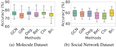
The results of this experiment inspired us to design a centrality-based framework for graph-level tasks, which touches on the essence more than existing pipelines, but also poses challenges. Since the applicability of different centrality to different types of graph data varies, manually selecting the most appropriate centrality can be very labor-intensive. Thus we would like to learn an adaptive centrality to synthesize the information provided by different centrality.
First, we construct a centrality matrix CGi ∈ Rni×s collecting various centrality measures for each graph Gi, where s denotes the number of initial centrality measures. Subsequently, a trainable weight vector w ∈ Rs is used to measure the overall importance of each centrality. Specifically, we let each element in w weight each column in CGi , as CGi = [w[1]CGi [:, 1], ...,w[s]CGi [:, s]]. This allows the model to initially learn how much information each centrality should provide to the subsequent process. Then we apply normalization to the centrality matrix due to the different scales of the centrality measures, which enhance model stability, i.e., ˆCGi = CGi -µGi σGi . This involves calculating the mean µGi and variance σGi .
After this, to further extract the information in the centrality matrix as well as the importance of each centrality and the interactions between them, we designed a centrality attention mechanism:
where QGi = Wq ˆCGi , KGi = Wk ˆCGi , VGi = Wv ˆCGi , and d is the dimension of the hidden layer. Through this attention-based manner, we can better capture the data distribution among different centralities and effectively learn an adaptive centrality that accommodates various datasets.
In practice, we also employ multi-head self-attention to enhance the model's expressiveness, allowing the model to capture different aspects of node relationships:
where QhGi = Wh q ˆCGi , KhGi = Wh k ˆCGi , Vh Gi = Wh v ˆCGi , and dh is the dimension for head h. Finally, the outputs from all heads are concatenated and projected through a linear transformation to produce the final adaptive centrality representation:
whereWO ∈ R∑Hi=1 di×d is a learnable weight matrix for the output transformation.
The adaptive centrality ΞGi ∈ RnGi ×d modulates the importance of nodes in the final representation. The final graph embedding zGi is computed as the weighted sum of the adaptive centrality, expressed as follows:
The choice of HGi offers considerable flexibility. It can be derived from various approaches, such as the node embeddings learned by a GNN or even the initial node feature vectors themselves. The function gΨ also provides a flexible mechanism for integrating the learned centrality ΞGi with node embeddings to produce the final graph embedding. It can take various forms: for instance, it could be a simple linear transformation that directly converts ΞGi into a vector, which is then used to perform a weighted summation over the node embeddings. Alternatively, it could act as a mapping function that applies the Hadamard product between ΞGi and HGi , followed by a summation.
In summary, the flexibility in the choice of gΨ and HGi allows for adapting the centrality-based method to different scenarios, leveraging either learned representations from GNN models or raw feature inputs, depending on the needs of the task or the dataset characteristics. Moreover, our ACGL framework can incorporate other graph learning strategies, making it a highly adaptable and extensible method for a wide range of graph-based tasks.
2.4 Overall Framework
For better understanding, we briefly describe our proposed method in this subsection
where MΦ denotes the adaptive centrality learning process, which contains the initial construction of CGi , Equations (16) and (17). Φ is the set of all trainable parameters, similarly we have W and Ψ for corresponding processes. fW is an encoder chosen from linear layer, MLP, and GNNs. When equipped with GNNs, the model can be viewed as ACRead, while it becomes ACGL when choosing a linear layer or an MLP.
For a comprehensive understanding of computational efficiency, we analyze the time complexity of our proposed method for N graphs. The GNN encoder, responsible for transforming initial node features into node embeddings, exhibits a time complexity of O(N(nd+ |E|)(Ld+d0)). Here, n denotes the maximum number of nodes, |E| represents the maximum number of edges, d0 is the dimension of initial node features, d indicates the maximum hidden dimension, and L represents the number of GNN layers. This complexity encompasses both propagation and aggregation operations across all layers. In the adaptive centrality mechanism, the query, key, and value mapping layers utilize a hidden dimension dh (where dh ≪ d), resulting in a complexity of O(Nnsdh). The attention computations, including score calculations and matrix multiplications, contribute a complexity of O(Nhn2dh) (where s ≪ dh and h represents the number of attention heads). Given that the batch size n remains smaller than the hidden dimension d during training, the overall time complexity maintains at O(N(nd + |E|)(Ld + d0)). Notably, the computational overhead introduced by our approach is minimal in the context of the complete framework. For the detailed training times, please refer to Appendix B.5.
3 Expreiments
This section presents experiments to evaluate our proposed methods. We first introduce experimental settings, followed by performance analysis on graph classification and representation learning tasks. We also conduct ablation studies and provide visualizations. Detailed experimental settings are provided in the Appendix B.
3.1 Experiments Setting
Datasets. We utilize 8 graph-level datasets, comprising 2 social network datasets (IMDB-B and IMDB-M) and 6 smallmolecule chemical datasets (MUTAG, DD, PROTEINS, NCI1, Mutagenicity and OGBG-Molhiv). All datasets were collected from the TU datasets [Morris et al., 2020] and open graph benchmark repositories [Hu et al., 2020].
Backbone and Baseline. This paper employed six commonly used supervised GNN frameworks: basic GNNs (GCN [Welling and Kipf, 2017], GraphSAGE [Hamilton et al., 2017], SGC [Wu et al., 2019]), and three more expressive GNNs (GAT [Veliˇckovi´c et al., 2018], GIN [Xu et al., 2018], and GUNet [Gao and Ji, 2019]). Besides, two unsupervised GNNs (InfoGraph [Sun et al., 2019] and GraphCL [You et al., 2020]) are also used in this article. Additionally, we selected 11 readout functions as baselines, including simple readouts (Sum, Mean, Max), as well as learnable readouts (Attention [Li et al., 2016], Set2Set [Vinyals et al., 2016], Deep Sets [Zaheer et al., 2017], SRead [Lee et al., 2021], Janossy MLP [Buterez et al., 2022]), sequence-based readouts (Set Transformer, and Janossy GRU [Buterez et al., 2022]), and kernelbased methods (KerRead [Yu et al., 2024]).
Parameter Settings. In this paper, we utilized 9 different centrality measures as the initial centrality features, including: degree centrality, betweenness centrality, closeness centrality, PageRank, hubs, authorities, load centrality, harmonic centrality, and bridge centrality. These centrality measures offer varied insights into node importance and influence within the graph, forming the foundation for our adaptive centrality module. Additional experimental settings and implementation details can be found in the Appendix.
3.2 Experimental Results Analysis
Graph Classification. We conducted a comprehensive graph classification task using 11 readout functions across 6
backbone models. The results for 7 smaller datasets are compared in Tables 1 and Appendix B.4, while the results for a larger dataset are shown in Table 2 to ensure the reliability of our findings. Based on these tables, we observed the following phenomena: (i) ACRead exhibited superior performance, outperforming the previously strongest baseline, KerRead, by an average of 5.1%, 4.2%, and 5.5% on GAT, GUNet, and SGC, respectively. (ii) ACRead demonstrated strong stability. While other readouts performed poorly on GAT and SGC, ACRead maintained consistent performance across all backbones. Specifically, the largest performance difference for ACRead across the 6 backbones was only 3.5%, whereas other readouts showed performance gaps as large as 8.1%. (iii) ACRead's effectiveness persisted even on weaker models. For instance, even on the less expressive SGC model, ACRead outperformed most readouts applied to stronger backbones like GUNet. These results highlight the robustness and effectiveness of ACRead across various models and datasets.
GraphRepresentationLearning. The graph clustering results are shown in Table 3, which provides a comparison of 11 readout functions across two unsupervised GNN backbones, InfoGraph and GraphCL, and we can find that: (i) ACRead consistently outperforms other readouts. It achieves the highest performance in terms of both ACC and NMI across multiple datasets, particularly on MUTAG, DD, and NCI1. (ii) ACRead demonstrates strong adaptability across datasets. It maintains robust performance across molecular datasets and social network datasets, confirming its versatility. (iii) While other readouts show significant performance variation depending on the dataset and backbone, ACRead maintains stable results across both InfoGraph and GraphCL. For example, with the InfoGraph backbone, ACRead's NMI ranges from 19.2 to 36.9 across datasets, which is comparatively lower than the fluctuations observed in other methods.
Selection of gΨ and HGi . To validate the effectiveness of our proposed ACGL framework, we experimented with various configurations of HGi and gΨ to assess their performance in graph classification. As shown in Table 4, we conducted experiments on four datasets using three different HGi and two different gΨ. The operators ⊙ and Linear respectively represent the Hadamard product using the learned Υ ∈ RnGi ×d directly, or a linear transformation into a vector of size nGi × 1 followed by weighted summation. We observed the following phenomena: (i) More complex HGi typically leads to better results. Using the initial features XGi as the starting vector already yields performance comparable to Table 1. However, it's clear that applying an MLP transformation on XGi yields even better results, and the best performance is achieved when HGi is learned using GNNs for weighted summation, as evidenced in Tables 1. (ii) The ⊙ operator outperforms the simple linear summation, as it not only applies weights to each node but also to each dimension, enabling the capture of more information.
| Backbone | Method | MUTAG | DD | PROTEINS | NCI1 | Mutagenicity | IMDB-B | IMDB-M | Avg. |
|---|---|---|---|---|---|---|---|---|---|
| GCN [Welling and Kipf, 2017] | Sum | 86.7 (5.5) | 68.8 (4.7) | 73.9 (3.5) | 75.8 (2.3) | 78.0 (1.8) | 69.9 (4.3) | 48.1 (4.1) | 71.6 |
| Max | 81.8 (9.7) | 72.8 (4.3) | 66.0 (5.7) | 72.4 (3.9) | 79.6 (1.7) | 71.2 (4.1) | 46.7 (4.3) | 70.1 | |
| Mean | 87.2 (7.3) | 71.1 (3.0) | 68.1 (4.1) | 73.6 (1.8) | 78.5 (2.2) | 71.1 (3.3) | 48.7 (3.8) | 71.2 | |
| Set2set | 84.0 (4.2) | 74.2 (4.9) | 72.5 (4.0) | 80.9 (1.9 | 82.0 (0.9) | 69.3 (4.3) | 48.5 (3.8) | 73.1 | |
| Attention | 87.2 (4.4) | 71.4 (4.0) | 70.5 (3.5) | 74.5 (2.6) | 80.2 (2.3) | 72.0 (4.6) | 47.1 (5.5) | 71.8 | |
| Deep Sets | 84.6 (4.9) | 73.6 (3.3) | 75.5 (5.3) | 76.2 (1.9) | 78.2 (1.1) | 72.0 (2.9) | 48.5 (2.8) | 72.7 | |
| SRead | 86.1 (5.6) | 68.8 (3.2) | 74.1 (5.0) | 75.8 (2.0) | 78.4 (1.9) | 70.4 (4.7) | 47.6 (3.9) | 71.6 | |
| Set Transformer | 84.6 (6.0) | 69.7 (3.9) | 71.7 (5.8) | 80.7 (2.6) | 82.0 (1.7) | 72.1 (3.0) | 48.3 (1.7) | 72.7 | |
| Janossy MLP | 76.7 (11.4) | 54.0 (3.4) | 65.6 (4.0) | 71.8 (2.1) | 74.6 (1.7) | 67.8 (3.3) | 48.3 (3.1) | 65.5 | |
| Janossy GRU | 84.6 (7.7) | 58.6 (0.4) | 59.5 (0.2) | 80.2 (1.6) | 73.5 (10.8) | 69.3 (3.6) | 46.1 (6.6) | 67.4 | |
| KerRead | 88.3 (6.1) | 77.8 (3.0) | 75.9 (2.8) | 82.6 (2.0) | 82.6 (2.0) | 72.5 (2.4) | 49.0 (2.9) | 75.5 | |
| ACRead | 89.9 (6.9) | 78.2 (4.6) | 76.1 (5.3) | 83.2 (2.3) | 82.0 (2.6) | 72.9 (5.2) | 49.7 (4.8) | 76.0 | |
| GAT [Veli ˇckovi ´c et al., 2018] | Sum | 76.0 (8.8) | 73.6 (3.9) | 73.6 (3.1) | 70.9 (3.0) | 75.0 (2.1) | 50.0 (0.0) | 34.7 (2.3) | 64.8 |
| Max | 75.5 (8.4) | 74.3 (4.1) | 66.9 (5.0) | 62.0 (3.5) | 73.3 (2.9) | 50.0 (0.0) | 33.3 (0.0) | 62.2 | |
| Mean | 74.9 (9.7) | 70.3 (4.2) | 70.0 (5.4) | 69.1 (2.2) | 75.8 (2.6) | 50.0 (0.0) | 33.7 (1.4) | 63.4 | |
| Set2set | 76.0 (10.9) | 75.2 (5.4) | 72.6 (4.1) | 73.5 (1.6) | 78.7 (2.4) | 50.0 (0.0) | 33.3 (0.0) | 65.6 | |
| Attention | 78.7 (8.1) | 67.7 (4.2) | 71.4 (5.4) | 69.5 (2.2) | 76.9 (1.8) | 50.0 (0.0) | 33.3 (0.0) | 63.9 | |
| Deep Sets | 74.0 (12.0) | 72.8 (4.6) | 74.2 (4.9) | 72.0 (1.7) | 74.7 (1.3) | 50.0 (0.0) | 33.3 (0.0) | 64.4 | |
| SRead | 74.4 (7.8) | 70.0 (4.5) | 73.8 (4.0) | 70.2 (3.1) | 74.1 (1.8) | 50.2 (0.6) | 34.4 (2.3) | 63.9 | |
| Set Transformer | 74.0 (8.6) | 66.8 (4.0) | 73.4 (5.2) | 72.9 (2.3) | 79.6 (1.8) | 50.0 (0.0) | 33.3 (0.0) | 64.3 | |
| Janossy MLP | 74.4 (7.4) | 52.3 (3.9) | 65.0 (4.7) | 68.4 (1.8) | 71.4 (1.7) | 50.0 (0.0) | 33.3 (0.0) | 59.3 | |
| Janossy GRU | 75.5 (9.1) | 69.9 (5.0) | 59.5 (0.3) | 75.5 (3.1) | 65.3 (11.2) | 50.0 (0.0) | 33.3 (0.0) | 62.7 | |
| KerRead | 79.1 (8.4) | 76.4 (4.5) | 77.4 (3.5) | 76.0 (1.2) | 80.2 (1.4) | 51.4 (1.5) | 34.2 (1.8) | 67.4 | |
| ACRead | 88.2 (5.3) | 76.9 (3.5) | 75.2 (4.1) | 81.2 (2.4) | 80.5 (2.3) | 64.9 (4.8) | 40.3 (3.3) | 72.5 | |
| GIN [Xu et al., 2018] | Sum | 85.1 (5.9) | 70.6 (3.7) | 69.4 (5.0) | 73.5 (1.4) | 76.0 (1.5) | 67.0 (3.4) | 48.2 (3.7) | 71.0 |
| Max | 84.4 (5.6) | 72.1 (4.1) | 66.9 (4.9) | 72.6 (2.3) | 76.6 (1.2) | 67.7 (3.8) | 48.1 (4.2) | 71.2 | |
| Mean | 82.0 (8.6) | 73.0 (4.0) | 69.4 (5.5) | 74.4 (1.8) | 76.6 (1.7) | 66.7 (3.6) | 48.3 (3.9) | 70.5 | |
| Set2set | 86.1 (5.1) | 72.0 (4.7) | 73.0 (3.2) | 73.9 (2.6) | 76.9 (1.4) | 67.0 (3.4) | 49.1 (4.4) | 72.6 | |
| Attention | 85.4 (4.2) | 72.8 (3.9) | 73.5 (4.4) | 74.2 (1.9) | 77.0 (2.2) | 66.7 (3.8) | 49.3 (4.0) | 72.8 | |
| Deep Sets | 87.1 (6.2) | 73.9 (4.0) | 74.1 (4.3) | 75.8 (1.5) | 76.9 (1.8) | 69.8 (3.2) | 49.5 (3.8) | 73.5 | |
| SRead | 84.4 (7.0) | 67.4 (4.3) | 73.1 (5.5) | 73.8 (2.4) | 75.6 (1.6) | 66.3 (2.8) | 48.5 (3.1) | 71.0 | |
| 85.1 (6.9) | 70.5 (3.7) | 72.4 (3.8) | 72.6 (2.4) | 78.2 (1.9) | 68.2 (3.0) | 48.4 (4.6) | 72.2 | ||
| Set Transformer Janossy MLP | 75.6 (9.9) | 55.5 (3.5) | 64.9 (3.6) | 73.6 (2.1) | 75.0 (1.8) | 65.5 (3.2) | 47.4 (5.1) | 65.1 | |
| Janossy GRU | 82.1 (8.8) | 57.4 (2.1) | 67.5 (4.8) | 72.9 (3.5) | 72.8 (3.8) | 65.2 (3.5) | 47.8 (6.7) | 66.8 | |
| KerRead | 87.5 (5.2) | 77.9 (4.3) | 76.6 (3.7) | 78.2 (2.8) | 79.0 (1.5) | 70.3 (2.0) | 50.0 (4.1) | 74.3 | |
| ACRead | 87.8 (5.4) | 76.8 (4.3) | 76.9 (4.6) | 82.4 (3.2) | 82.2 (2.3) | 71.5 (3.5) | 50.6 (3.4) | 75.5 |
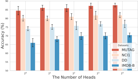
The Number of Heads. Figure 2 illustrates the relationship between the number of heads and the accuracy across four datasets. The x-axis represents the number of heads, scaled exponentially (from 20 to 24 ), while the y-axis shows the corresponding accuracy for each dataset. In general, accuracy tends to increase with a higher number of heads across all datasets. This trend suggests that increasing the number of attention heads in the model contributes positively to classification performance, reflecting improved representation learning. However, the performance improvement diminishes as the number of heads increases from 23 to 24 . While the initial increase in heads (from 20 to 23 ) leads to notable accuracy gains across all datasets, the jump from 23 to 24 shows a much smaller improvement. This trend suggests that after a certain point, adding more heads yields diminishing returns, possibly because the model reaches a saturation point where further splitting attention no longer substantially enhances the representation learning.
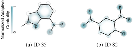
Visiualization. The normalized adaptive centrality scores, scaled between (0, 1), are visualized with darker colors representing nodes of greater influence on the graph embedding. We randomly selected two samples from the MUTAG dataset, as shown in Figure 3, where the goal is to predict mutagenicity in Salmonella typhimurium. Both samples activate the mutagenic gene. Adaptive centrality identified functional groups like F and Cl as important, while carbon atoms in the benzene ring were less significant. This highlights adaptive centrality's ability to capture node importance, offering insights for future graph-level tasks.
| Dataset | Readout | GCN | GIN | GraphSAGE | GAT | GUNet | SGC | Avg |
|---|---|---|---|---|---|---|---|---|
| OGBG-Molhiv | Sum | 60.9 (2.9) | 71.3 (1.7) | 58.3 (2.3) | 62.3 (2.1) | 59.0 (1.7) | 59.7 (2.1) | 61.9 |
| Max | 58.4 (2.3) | 71.8 (2.0) | 66.9 (3.6) | 67.7 (2.0) | 66.7 (4.4) | 66.1 (3.2) | 66.3 | |
| Mean | 57.4 (1.8) | 70.9 (2.4) | 51.0 (2.2) | 60.4 (2.3) | 50.3 (1.0) | 50.3 (0.7) | 56.7 | |
| Set2set | 66.8 (1.8) | 70.9 (1.3) | 59.4 (1.8) | 65.7 (2.0) | 56.7 (2.1) | 58.0 (1.1) | 62.9 | |
| # Graphs: 41,127 | Attention | 62.0 (1.7) | 70.4 (1.5) | 51.1 (1.9) | 58.5 (3.0) | 51.0 (1.6) | 51.8 (2.2) | 57.5 |
| # Features: 9 | Deep Sets | 63.3 (2.0) | 52.9 (1.0) | 53.1 (0.8) | 62.2 (2.2) | 53.4 (1.4) | 52.7 (1.0) | 56.3 |
| # Classes: 2 | SRead | 63.0 (1.4) | 70.9 (2.5) | 57.2 (1.2) | 63.2 (2.9) | 59.1 (3.4) | 51.8 (2.2) | 60.9 |
| Avg. # Nodes: 25.5 | Set Transformer | 72.2 (1.6) | 71.2 (1.3) | 61.3 (1.4) | 69.4 (1.5) | 61.8 (2.2) | 69.2 (2.1) | 67.5 |
| Avg. # Edges: 27.5 | Janossy MLP | 52.4 (0.6) | 50.0 (0.1) | 50.0 (0.1) | 51.5 (1.2) | 50.0 (0.0) | 50.0 (0.0) | 50.7 |
| Janossy GRU | 71.1 (1.4) | 67.9 (2.6) | 68.1 (2.4) | 69.1 (1.2) | 67.1 (1.9) | 68.1 (2.2) | 68.6 | |
| KerRead | 72.5 (1.6) | 72.2 (1.5) | 67.1 (1.2) | 70.4 (0.7) | 67.9 (2.6) | 68.9 (2.1) | 69.8 | |
| ACRead | 72.9 (1.4) | 73.1 (1.9) | 69.2 (1.4) | 70.6 (1.9) | 69.5 (1.6) | 69.4 (1.8) | 70.6 |
| Backbone | Readout | MUTAG | DD | PROTEINS | NCI1 | Mutagenicity | IMDB-B | IMDB-M | |||||||
|---|---|---|---|---|---|---|---|---|---|---|---|---|---|---|---|
| ACC | NMI | ACC | NMI | ACC | NMI | ACC | NMI | ACC | NMI | ACC | NMI | ACC | NMI | ||
| Sum | 71.3 | 14.1 | 59.7 | 2.6 | 60.4 | 2.6 | 56.6 | 1.3 | 56.4 | 1.7 | 62.3 | 4.4 | 40.8 | 2.2 | |
| Max | 80.9 | 25.6 | 60.8 | 4.7 | 61.7 | 2.8 | 60.4 | 3.3 | 57.2 | 1.6 | 61.1 | 4.7 | 38.9 | 2.2 | |
| Mean | 71.3 | 14.1 | 56.5 | 2.2 | 62.4 | 3.4 | 56.8 | 1.4 | 60.0 | 3.5 | 63.1 | 5.2 | 41.0 | 2.4 | |
| Set2set | 74.5 | 17.5 | 63.2 | 6.0 | 62.5 | 3.2 | 59.0 | 2.4 | 62.7 | 4.3 | 62.9 | 5.1 | 40.5 | 3.2 | |
| InfoGraph Attention | 80.3 | 24.4 | 55.2 | 1.0 | 59.9 | 2.4 | 57.3 | 1.6 | 63.3 | 5.1 | 62.9 | 5.0 | 40.3 | 1.8 | |
| [Sun et al., Deep Sets | 76.1 | 33.5 | 60.9 | 3.2 | 62.3 | 3.2 | 57.8 | 1.9 | 60.5 | 3.7 | 62.4 | 4.6 | 41.3 | 2.2 | |
| 2019] SRead | 79.3 | 31.7 | 60.4 | 3.6 | 59.5 | 2.0 | 58.3 | 2.0 | 61.1 | 4.2 | 62.6 | 4.6 | 41.5 | 2.5 | |
| Set Transformer | 73.9 | 16.9 | 70.3 | 13.0 | 59.8 | 2.6 | 60.9 | 3.6 | 65.2 | 6.4 | 63.6 | 5.4 | 41.5 | 1.9 | |
| Janossy MLP | 62.8 | 11.5 | 55.4 | 1.3 | 58.8 | 0.4 | 59.4 | 3.0 | 62.4 | 7.3 | 62.2 | 4.3 | 41.9 | 2.1 | |
| Janossy GRU | 70.7 | 26.0 | 58.6 | 0.0 | 59.4 | 0.0 | 58.1 | 0.0 | 62.3 | 0.1 | 50.1 | 0.0 | 42.3 | 3.5 | |
| KerRead | 83.5 | 36.4 | 74.8 | 20.5 | 63.4 | 6.3 | 61.8 | 3.8 | 65.7 | 7.0 | 63.5 | 5.3 | 42.8 | 2.6 | |
| ACRead | 84.8 | 36.9 | 75.1 | 21.2 | 65.1 | 6.9 | 63.2 | 4.1 | 66.2 | 7.8 | 64.2 | 6.1 | 43.1 | 3.2 | |
| Sum | 73.9 | 16.9 | 66.0 | 8.3 | 64.8 | 4.7 | 57.2 | 1.6 | 61.5 | 3.7 | 57.6 | 2.4 | 42.5 | 3.0 | |
| Max | 79.3 | 21.8 | 59.1 | 3.1 | 64.4 | 4.5 | 58.7 | 2.2 | 61.1 | 3.7 | 62.6 | 5.0 | 39.9 | 3.4 | |
| Mean | 73.9 | 16.9 | 66.3 | 8.7 | 64.4 | 4.5 | 55.2 | 0.8 | 61.6 | 3.4 | 61.6 | 4.0 | 42.9 | 3.3 | |
| Set2set | 70.7 | 17.5 | 60.7 | 2.5 | 63.4 | 3.2 | 58.3 | 2.6 | 63.6 | 6.6 | 64.8 | 6.4 | 43.8 | 3.8 | |
| GraphCL Attention | 76.1 | 24.3 | 55.8 | 0.5 | 62.0 | 2.1 | 57.6 | 2.3 | 61.1 | 3.1 | 60.9 | 4.5 | 39.9 | 3.5 | |
| [You et al., Deep Sets | 75.0 | 18.2 | 58.7 | 4.1 | 61.2 | 2.5 | 57.8 | 2.1 | 64.5 | 6.2 | 59.6 | 3.3 | 41.8 | 2.8 | |
| 2020] SRead | 76.6 | 24.9 | 68.1 | 8.9 | 65.1 | 5.0 | 57.1 | 2.1 | 62.2 | 5.8 | 63.9 | 8.6 | 43.9 | 4.0 | |
| Set Transformer | 79.8 | 32.2 | 53.7 | 0.3 | 58.3 | 1.7 | 55.7 | 1.0 | 61.4 | 4.0 | 59.6 | 4.2 | 41.9 | 2.5 | |
| Janossy MLP | 72.3 | 9.8 | 52.0 | 0.2 | 62.1 | 2.3 | 54.3 | 0.7 | 64.1 | 6.0 | 60.7 | 3.4 | 42.3 | 2.9 | |
| Janossy GRU | 81.4 | 33.8 | 55.4 | 0.6 | 65.1 | 4.7 | 56.2 | 1.2 | 56.6 | 1.3 | 57.7 | 2.3 | 44.7 | 3.0 | |
| KerRead | 83.5 | 34.1 | 75.4 | 18.7 | 70.9 | 11.2 | 58.8 | 2.8 | 64.2 | 6.1 | 64.4 | 6.5 | 45.0 | 3.6 | |
| ACRead | 84.1 | 35.8 | 76.2 | 19.2 | 71.0 | 11.3 | 61.3 | 4.1 | 66.2 | 7.9 | 65.1 | 6.9 | 46.0 | 4.1 | |
| HGi | gΨ | MUTAG | DD | PROTEINS | IMDB-M |
|---|---|---|---|---|---|
| XGi | ⊙ | 84.1 (7.2) | 75.2 (5.1) | 74.1 (4.3) | 46.3 (5.2) |
| Linear(XGi ) | ⊙ | 86.2 (8.5) | 76.2 (5.3) | 76.4 (4.5) | 48.3 (5.1) |
| MLP(XGi ) | ⊙ | 87.7 (8.1) | 78.4 (5.8) | 76.2 (4.9) | 49.3 (4.9) |
| XGi | Linear | 85.1 (7.3) | 74.1 (6.2) | 75.3 (5.1) | 45.9 (3.6) |
| Linear(XGi ) | Linear | 86.1 (7.2) | 75.3 (5.5) | 76.1 (4.5) | 47.1 (4.9) |
| MLP(XGi ) | Linear | 87.5 (6.1) | 77.5 (5.7) | 75.9 (4.6) | 48.1 (4.2) |
Supplementary Experiment Due to space constraints, additional crucial experiments are included in the appendices, including graph classification performance with GUNet, GraphSAGE, and SGC backbones (Appendix B.4), as well as training time analysis (Appendix B.5).
4 Conclusion
In this paper, we revisited the essence of message passing in graph-level tasks through the perspective of centrality, uncovering that it primarily operates as a weighted summation with degree-based centrality, which represents a single-view of node centrality. Building on this insight, we introduced a novel graph-level learning method with a more generalizable form of centrality-adaptive centrality, which integrates multiple views of node centrality and is utilized to build a novel readout function, called Adaptive Centrality-based Readout (ACRead). ACRead was applied to six supervised and two unsupervised GNN backbones, consistently outperforming existing readout methods across eight graph datasets. Furthermore, the approach could also perform as an individual graph-level learning framework without GNNs, called Adaptive Centrality-based Graph Learning (ACGL), which still achieved competitive performance by effectively combining different views of node centrality.
Acknowledgements
This work was supported by the National Natural Science Foundation of China (Grant Nos. 62202422 and 62372408).
Contribution Statement
Jiajun Yu and Zhihao Wu contributed equally as co-first authors.
@inproceedings{ijcai2025p399,
  title     = {A Centrality-based Graph Learning Framework},
  author    = {Yu, Jiajun and Wu, Zhihao and Lu, Jielong and Wang, Tianyue and Wang, Haishuai},
  booktitle = {Proceedings of the Thirty-Fourth International Joint Conference on
               Artificial Intelligence, {IJCAI-25}},
  publisher = {International Joint Conferences on Artificial Intelligence Organization},
  editor    = {James Kwok},
  pages     = {3588--3596},
  year      = {2025},
  month     = {8},
  note      = {Main Track},
  doi       = {10.24963/ijcai.2025/399},
  url       = {https://doi.org/10.24963/ijcai.2025/399},
}
TY - CPAPER TI - A Centrality-based Graph Learning Framework AU - Yu, Jiajun AU - Wu, Zhihao AU - Lu, Jielong AU - Wang, Tianyue AU - Wang, Haishuai T2 - Proceedings of the Thirty-Fourth International Joint Conference on Artificial Intelligence, IJCAI-25 PB - International Joint Conferences on Artificial Intelligence Organization PY - 2025 SP - 3588 EP - 3596 DO - 10.24963/ijcai.2025/399 UR - https://doi.org/10.24963/ijcai.2025/399 ER -Copied
Machine-readable versions of this paper, for tools and AI agents:





