Time-Frequency Disentanglement Boosted Pre-Training: A Universal Spatio-Temporal Modeling Framework

1 Introduction

Spatio-temporal graph learning is not only a powerful tool for understanding complex urban systems but also an intelligent measure for modeling the evolution of human behavior and natural environment [Shi et al., 2023; Zhang et al., 2024]. Despite the advances in spatio-temporal graph learning, most existing methods are typically designed for specific tasks and assume access to large volumes of high-quality data [Wang et al., 2020; Liu et al., 2025a; Miao et al., 2024a; Liao et al., 2024; Miao et al., 2025]. However, this assumption often breaks down in numerous real-world urban environments, particularly in newly developed areas [Wang et al., 2019; Deng et al.,

∗Prof. Yang Wang and Dr. Xu Wang are the corresponding authors. Primary Contact: Dr. Xu Wang.

2024]. These areas frequently possess few or no pre-deployed sensors, making it difficult to collect sufficient data for training robust models. This dilemma makes us think about how to carry out effective spatio-temporal graph few-shot learning in such data-scarce areas. Furthermore, as smart applications become more ubiquitous, the demand for deploying diverse services continues to grow. Developing, training, and maintaining separate spatio-temporal models for each service or task is not only resource-intensive but also significantly slows down the deployment of intelligent urban solutions [Zhang et al., 2023]. Therefore, there is a pressing need for the generalization of spatio-temporal models enabling a universal model to adapt to different tasks with minimal retraining.

As a promising cross-domain and cross-task knowledge transfer approach, transfer learning, dominated by pre-training techniques, aims to utilize the knowledge learned from data-rich sources domain to perform various downstream tasks in a data-scarce target domain [Zhuang et al., 2020; Liu et al., 2025b]. In recent years, researchers have realized the significant potential of pre-trained spatio-temporal models for cross-city few-shot learning and cross-task generalization, and have proposed a variety of solutions [Shao et al., 2022; Jin et al., 2023a]. For example, TPB [Liu et al., 2023] utilizes a pre-trained traffic patch encoder to project raw traffic data from data-rich cities into a high-dimensional space. STGP [Hu et al., 2024] proposes a prompt-enhanced transfer learning framework capable of adapting to diverse tasks in data-scarce domains. Existing pre-trained spatio-temporal models basically inherited the idea of Masked Autoencoder in STEP [Shao et al., 2022] and achieved superior performance, but we deeply find that there are still two critical challenges that have not yet been adequately addressed, constraining the development of more universal spatio-temporal models.

Challenge 1. Inadequate ability to represent spatiotemporal information in source domains. The existing models are based on self-supervised learning methods in the time domain [Shao et al., 2022], which neglects the complex and indispensable topological relationships in the spatial dimension in spatio-temporal data on the one hand, making the models lack the ability to model spatial information. On the other hand, just as important as the time domain are the temporal patterns in the frequency domain, whereas such potential but inherent trend information in spatio-temporal data has seldom been considered in spatio-temporal pre-training. Therefore, these two shortcomings severely limit the effective extraction of spatio-temporal information from the source domains.

Challenge 2. Deficient adaptability to target domains and tasks. Most of the approaches add specific modules for different downstream tasks for training in the fine-tuning stage [Liu et al., 2023]. This seemingly simple approach fails to pay attention to the individualized information of the graph structure in the target city on the one hand, leading to poor results even after fine-tuning the model, and on the other hand, it greatly reduces the model's generalizability and complicates the process of adapting the model to different tasks. Undoubtedly, improving the model's ability to adapt to target domains and downstream tasks will unleash the greater potential of pre-trained spatio-temporal models.

To effectively address the above challenges, we propose a Universal Spatio-Temporal Correlationship pre-training framework (termed USTC), for spatio-temporal modeling across different cities and tasks. In particular, for Challenge 1, we decouple the time- and frequency-domain patterns of trend and seasonality in the data respectively during pre-training. After patched masking, we introduce a stacked structure of Transformer and Graph Neural Network (GNN) in encoding the spatio-temporal information and apply contrastive learning to the encoded time- and frequency-domain information to maintain the consistency of the original signals. For Challenge 2, we propose a prompt generation module in the fine-tuning stage to mine the personalized information in each node on the target city, which is combined with the shared spatio-temporal representations learned by the pre-trained encoder to serve the downstream tasks, and we introduce a common decoder for the three mainstream spatio-temporal tasks (i.e., forecasting, imputation, and extrapolation) to extract the common semantics among the tasks and achieve cross-task generalization. The main contributions of our work lie in three aspects:

• ❶ Novel insight and framework: We innovatively construct a cross-city and cross-task spatio-temporal learning paradigm, and propose a time-frequency disentanglement boosted pretraining architecture called USTC, which enables the effective solution of spatio-temporal forecasting, imputation, and extrapolation with a universal model.
• ❷ Advisable methodologies: To enhance the spatiotemporal representations in pre-training, we decouple the time- and frequency-domain patterns of trend and seasonality in the data respectively, introduce the stacked structure of Transformer and GNN for spatio-temporal relationship extraction, and use contrastive learning for the encoded information to maintain the time-frequency consistency. To improve the adaptability of downstream tasks in fine-tuning, we propose a prompt generation module to mine personalized spatio-temporal patterns on the target city, which are integrated with the common spatio-temporal representations to collaboratively serve the downstream tasks.

❸ Compelling empirical results: We conduct extensive experiments on four real-world datasets, evaluating USTC on spatio-temporal forecasting, imputation, and extrapolation tasks. The results consistently demonstrate the superior performance of USTC across various scenarios.

2 Preliminaries

Definition 1. Spatio-Temporal Graph. A spatio-temporal graph can be denoted as G = (V, E,A) [Fang et al., 2023; Zhang et al., 2025a; Zhang et al., 2025b]. V is the set of nodes, N = |V| is the number of nodes, and E is the set of edges. A ∈ RN×N is the adjacency matrix of G, which describes the weights between nodes.

Definition 2. Spatio-Temporal Data. Spatio-temporal data contained in the spatio-temporal graph can be denoted as X ∈ RN×T×C , where N represents the number of nodes, T represents a time window, and C indicates the channel of inputs. And we donoted the spatio-temporal data of node i at time step t as Xit ∈ RC [Fang et al., 2024].

Problem 1. Spatio-Temporal Graph Transfer Learning. Given P data-rich source domains G source = {G source 1 , · · · , G source P } and a data-scarce target domain G target . The goal of spatio-temporal graph transfer learning is to pre-train a model on the data of G source to assimilate the relevant knowledge of the source domains, and fine-tune the model to adapt to the target domain G target by utilizing the knowledge acquired. The fine-tuned model is required to accomplish various spatio-temporal graph learning tasks.

Problem2. Forecasting. Given the historical spatio-temporal data of Th time steps from a target domain, the goal of the forecasting problem is to transfer the pre-trained function f(·) to forecast the future data of Tf time steps [Liu et al., 2024a; Miao et al., 2024b]. This task can be formulated as follows:

where X[Th+1:Th+Tf ] ∈ RN×Tf×C is the future data. Problem 3. Imputation. Given incomplete historical data of Th time steps from a target domain with missing values at certain time steps, the goal of imputation is to use the pretrained function f(·) to estimate and fill in the missing data. To characterize the missing situation of time step t, we create a 0-1 matrix as Rt ∈ {rij}N,C i,j=1 , where mij is defined as:

Therefore, the data with missing values of time step t can be defined as ˜Xt = Xt ⊙Rt, where Xt indicates the complete historical data of time step t. The problem of missing imputation can be formulated as follows:

where ˆX1:Th ∈ RN×Th×C represents the imputed data.

Problem 4. Extrapolation. Given the known historical spatiotemporal data of Th time steps from N observed nodes within a target domain, the goal of the extrapolation task is to utilize this information to predict the future data of Tf time steps of M unobserved nodes [Zhang et al., 2025c]. This task can be formulated as follows:

where XN+1:N+M Th+1:Th+Tf ∈ RM×Tf×C represents the future data of unobserved nodes.

3 Methodology

In this section, we present an overview of the proposed USTC framework, which contains two stages:

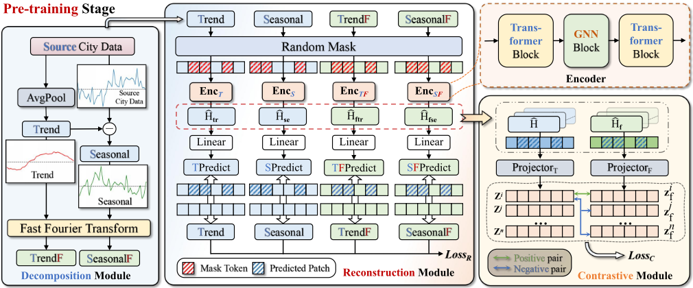
Stage 1. Pre-training. In this stage, we aim to learn robust knowledge from source domains. We introduce three novel modules as shown in Fig. 1. The first module is the Decomposition Module, which aims to process the source city data into four unique time-frequency information by leveraging average pooling and Fast Fourier Transform (FFT) techniques. The transformed information is then channeled as input into the subsequent Reconstruction Module. Within the Reconstruction module, inspired by [Shao et al., 2022; Liu et al., 2024c], we employ random masking and reconstruction strategies to learn the underlying temporal dynamics and spatial relationships. Furthermore, we introduce the Contrastive Module to encourage the encoder's capability to capture consistency across temporal and frequency domains.

Stage 2. Fine-tuning. The function of this stage is to adjust the model utilizing data from the target domain and task. Within this stage, the encoder, which was developed during the pre-training phase, is set to a fixed state. We have integrated a novel Prompt Generation Module, based on the consideration of node-specific knowledge that is ignored by the pre-trained encoder. To address this, we compute the difference between the encoder's input and output, and subsequently feed it into the prompt layer to generate node embeddings. These node embeddings are then concatenated with the hidden states extracted by the frozen encoder and introduced to the decoder. This approach enables the model to adapt to the distinct downstream tasks associated with the target city.

3.1 Pre-Training Stage

Decomposition Module

Inspired by AutoFormer [Wu et al., 2021a] and CoST [Woo et al., 2022], we utilize the decomposition strategy to learn the intricate temporal patterns, which separate spatio-temporal data into the trend and seasonal parts, which respectively reflect the long-term tendencies and the periodic seasonal variations inherent in the data. Specifically, we utilize the moving average to smooth out periodic fluctuations to yield the long-term trend component. Subsequently, by subtracting this trend component from the original data, we obtain the seasonal component. For the data Xi ∈ RT×C of node i, the aforementioned decomposition operation can be represented as follows:

where Xitr ,Xise ∈ RT×C denote the trend component and the seasonal component of Xi .

In addition, spatio-temporal data contains significant information in the frequency domain that is not evident in the time domain. To unearth this latent information, we employ the Fast Fourier Transform (FFT) to convert both trend and seasonal components into frequency domain, thereby capturing their spectral characteristics, which are delineated as follows:

where Fitr and Fise denote the frequency domain representations converted fromXitr and Xise , respectively.

Through the decomposition module, we have decomposed and transformed the spatio-temporal data into four sets of timefrequency components, which are represented as Xitr and Xise in the time domain, and Fitr and Fise in the frequency domain.

Reconstruction Module

The reconstruction module is designed to leverage masking and reconstruction strategies for the pre-training of the encoder [Shao et al., 2022]. Firstly, we perform random masking operations on the four sets of time-frequency data obtained from the decomposition module of the source cities. Formally, by taking the time domain as an example, we separate the input data of node i into P patches as Xi = {Si1 , . . . , SiP }.

And we use a vector M to indicate whether a patch is masked or not, for example, M i j = 1 indicates Sij is masked. Then, the unmasked part of the input is fed into four distinct encoders, and a learnable masked token Smt fills the place where the data is masked. Formally, the input can be denoted as:

where ˜Xi indicates the input sequence that has undergone the masking operation. Given that the structure of the four encoders is analogous, we will focus on trend data in the time domain as a representative example to explain. The encoder consists of three steps, each designed to process the input data and extract specific types of information. The initial step involves using a Transformer block, which is adept at capturing temporal dynamics within the input.

In the second step, a GNN block processes the relationships and interactions between different nodes, enabling the model to understand the spatial dependencies within the data.

where Ni is the set of neighboring nodes of node i. Similar to the first step, the third step utilizes a Transformer block to refine the temporal features that have been extracted, which helps to consolidate the temporal patterns identified earlier and integrate any spatial insights gained from the GNN module.

Here ˆHi denotes the output hidden embeddings of encoders, ˆXi indicates the reconstructed sequence of node i. W and b represent the weight matrix and bias vector associated with the linear transformation applied after the Transformer block's processing. Therefore, we have the following formula:

Then, the reconstruction loss can be formulated as follows:

We encourage the encoders to harness the intrinsic information within the time-frequency data by optimizing their parameters to minimize the reconstruction loss, enhancing the encoders' capacity to accurately reconstruct the partially masked input.

Contrastive Module

We introduce a contrastive module to reinforce time-frequency consistency within the data, which refers to the notion that the characteristics of a signal in the time domain should correspond to those in the frequency domain [Liu et al., 2024b; Zhang et al., 2022]. Here, we focus on the time-frequency consistency rather than the differences between trend and seasonal data. Therefore, we omit the subscripts tr and se and use ˆH to denote the time-domain hidden embeddings output by the encoders, and ˆHf to represent the frequency-domain hidden embeddings. To ensure the measurability of the distance between time- and frequency-domain embeddings, we project the time- and frequency-domain embeddings through two distinct projection operators, ProjectorT and ProjectorF, respectively. The formulation can be articulated as follows:

To maintain a set of time-domain data more similar to its corresponding frequency-domain data obtained through FFT, we use the NT-Xent Loss [Chen et al., 2020] to optimize the encoders, which can be formulated as:

where sim indicates the cosine similarity, and the negative samples Zjf are chosen fromN nodes randomly. This approach encourages the model to preserve the consistency between time- and frequency-domain embeddings. The total loss LP of pre-training stage is the weighted sum of LR and LC.

where α is a regularization weight for balancing this combined loss. Thus, the model is optimized to achieve time-frequency consistency while learning diverse representations.

3.2 Fine-Tuning Stage

Prompt Generate Module

The prompt generation module is designed to obtain node embeddings that capture the personalized information ignored by the encoders. We calculate the difference between the target city's data and the output derived from processing this data through the encoders, thereby identifying the information that the encoders have potentially missed. This information is then passed into the Prompt Layer to obtain the node embedding Pi . Formally, this process can be articulated as follows:

where IFFT is the Inverse Fast Fourier Transform. We hypothesize that the Euclidean distance between the node embeddings should correlate with the distances reflected by Dynamic Time Warping (DTW) [Berndt and Clifford, 1994]. To represent this similarity, we employ a Mean Squared Error (MSE) Loss, with the specific formula provided as follows:

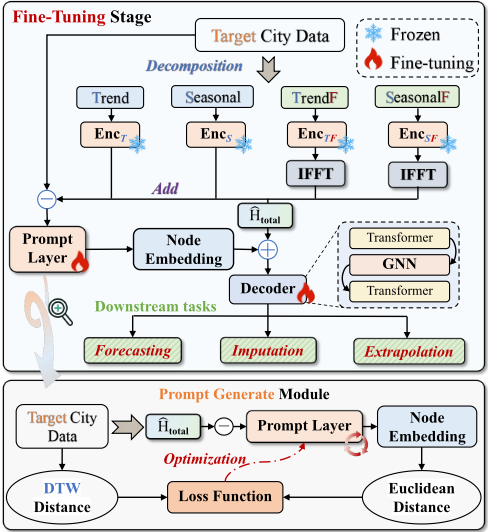
where DDTW is DTW distance between two time sequences, DEuc ies Euclidean distance between encoded embeddings, and n is the number of nodes in the target city. The finetuning of the prompt layer is guided by minimizing this loss, thereby ensuring that the node embeddings closely reflect the fine-grained personalized features of the target domain.

Fine-Tuning Module

In fine-tuning, our goal is to align the pre-trained encoders with the distinctive attributes of the target city. As illustrated in Fig. 2, we keep the encoders fixed while fine-tuning the prompt layer and decoder. The node embeddings P generated in the prompt generation module are concatenated with the hidden states ˆHtotal and then passed into the decoder. Echoing the encoders, the decoder also adopts a stacked structure to decouple the learned spatio-temporal representations. Formally:

MSE loss is utilized to optimize the decoder and prompt layer,

Finally, the total loss LF in fine-tuning is formalized as,

This fine-tuning procedure guarantees that the model can adeptly perform diverse downstream tasks within the target city, encompassing forecasting, imputation, and extrapolation.

Table 1: Statistical details of traffic datasets.

Datasets	PEMS-BAY	METR-LA	Chengdu	Shenzhen
# of Nodes	325	207	524	627
# of Edges	2,694	1,722	1,120	4,845
Interval	5 min	5 min	10 min	10 min
# of Time Step	52,116	34,272	17,280	17,280
Mean	61.7768	58.2749	29.0235	31.0092
Std	9.2852	13.1280	9.6620	10.9694

4 Experiments

4.1 Experimental Setup

Datasets. Four real-world widely used datasets are employed to evaluate our proposed framework, including PEMS-BAY, METR-LA [Li et al., 2018], Chengdu, and Shenzhen. These datasets comprise several months of traffic flow information, with the statistics listed in Table 1.

Few-Shot Transfer Learning Setting. Our framework is evaluated using a few-shot fine-tuning setting that aligns with [Lu et al., 2022; Liu et al., 2023]. The dataset is divided into three parts: pre-training data from three cities, few-shot fine-tuning data, and testing data from the other city. We use the comprehensive data from three cities for pre-training and select one city's data for both few-shot fine-tuning and testing. For instance, if Shenzhen is the city chosen for fine-tuning, the complete datasets from PEMS-BAY, METR-LA, and Chengdu are used for pre-training. A three-day dataset from Shenzhen is allocated for few-shot fine-tuning, while the rest of the data in Shenzhen is reserved for testing. We consider three classic tasks, including: 1) forecasting, predicting the future 1-hour data based on 1-day historical data. 2) imputation, forecasting the missing values within a given time window. 3) extrapolation, forecasting the future data of unobserved nodes, whose historical data is unknown. We use two widely used regression metrics: Mean Absolute Error (MAE) and Root Mean Squared Error (RMSE).

Baselines. We compare our model with 18 baseline models across three categories, which are listed as follows,

• ❶ Statistical Methods: HA and ARIMA calculate the statistical properties of input data to predict future signals. MEAN calculates the average value of the input and uses it to complete missing data. KNN completes missing data with the average value of its neighbors.
• ❷ Typical Deep-learning Methods: DCRNN [Li et al., 2018], ICREASE [Zheng et al., 2023], GWN [Wu et al., 2019], DSTAGNN [Lan et al., 2022], and FOGS [Rao et al., 2022] are classical models for spatiotemporal prediction. To apply them in the transfer learning scenario, we optimize them using the Reptile [Nichol et al., 2018] meta-learning framework.
• ❸ Transfer-learning Models: AdaRNN [Du et al., 2021], ST-GFSL [Lu et al., 2022], DASTNet [Tang et al., 2022], TPB [Liu et al., 2023], IGNNK [Wu et al., 2021b], SATCN [Wu et al., 2021c], TransGTR [Jin et al., 2023b], GPD [Yuan et al., 2024], and STGP [Hu et al., 2024] represent the cutting-edge in time series or spatio-temporal forecasting within the domain of transfer learning.

Notably, the conventional deep-learning methods are implemented with Reptile framework, which is a meta-learning Model Target City Chengdu Dataset Shenzhen Dataset Metrics MAE(↓)

	Target City	METR-LA								PEMS-BAY								RMSE(↓)
Model	Metrics Horizon	MAE(↓)			RMSE(↓)					MAE(↓)
		10 min	30 min	60 min	avg.	10 min	30 min	60 min	avg.	10 min	30 min	60 min	avg.	10 min	30 min	60 min	avg.
HA ARIMA	Target Only	3.62	4.23	5.13	4.33	7.33	8.56	10.17	8.69	2.42	2.89	3.70	3.00	5.46	6.52	8.25	6.74
DCRNN		3.22	3.70	5.00	3.97	6.28	7.80	9.80	7.96	2.28	2.49	3.66	2.81	4.52	5.35	7.45	5.77
GWN	Reptile	3.01	3.65	4.67	3.78	5.62	7.16	8.96	7.25	1.83	2.43	3.36	2.54	3.36	4.71	6.59	4.89
		3.11	3.75	4.73	3.86	5.87	7.31	9.10	7.43	1.99	2.45	3.14	2.53	3.55	4.64	6.23	4.81
DSTAGNN		3.30	4.10	4.95	4.12	5.90	7.73	9.56	7.73	1.85	2.51	3.59	2.65	3.41	4.79	6.66	4.95
FOGS		3.26	4.11	4.88	4.08	5.95	7.50	9.47	7.64	1.89	2.38	3.37	2.55	3.49	4.54	6.01	4.68
AdaRNN	Transfer	3.05	3.68	4.51	3.75	5.66	7.15	8.60	7.14	1.79	2.33	3.04	2.39	3.38	4.60	5.98	4.65
ST-GFSL		3.00	3.79	4.58	3.79	5.72	7.21	8.67	7.20	1.77	2.20	2.95	2.31	3.27	4.50	5.92	4.56
DSATNet		3.03	3.66	4.51	3.73	5.70	7.15	8.78	7.21	1.64	2.16	2.88	2.23	3.26	4.36	5.89	4.50
TPB		3.07	3.80	4.66	3.84	5.69	7.03	8.52	7.08	1.62	2.12	2.83	2.19	3.24	4.33	5.76	4.44
TransGTR		3.01	3.64	4.44	3.70	5.60	7.12	8.49	7.07	1.60	2.13	2.79	2.17	3.04	4.35	5.68	4.36
GPD		2.96	3.58	4.29	3.61	5.58	6.90	8.21	6.90	1.72	2.18	2.69	2.20	3.19	4.26	5.60	4.35
STGP		2.97	3.54	4.23	3.58	5.48	6.77	8.19	6.81	1.74	2.13	2.70	2.19	3.21	4.18	5.46	4.28
USTC	Transfer	2.85	3.41	4.10	3.45	5.37	6.58	8.10	6.68	1.69	2.05	2.63	2.12	3.09	4.22	5.48	4.26

RMSE(↓)

MAE(↓)

RMSE(↓)

Horizon 10 min 30 min 60 min avg. 10 min 30 min 60 min avg. 10 min 30 min 60 min avg. 10 min 30 min 60 min avg.

HA Target Only 2.69

ARIMA

2.97

3.13

3.65 3.16 3.69

4.57

5.27 4.51 2.17

2.66

3.04 2.62 3.33

4.05

4.63 4.00

3.28

4.32 3.52 3.78

4.64

5.51 4.64 2.35

2.99

3.60 2.98 4.32

4.73

5.58 4.88

DCRNN

GWN

DSTAGNN

FOGS

2.31

3.16

3.96 3.14 3.33

4.55

5.42 4.43 1.94

2.57

3.07 2.53 2.84

3.81

4.52 3.72

2.19

2.81

3.21 2.74 3.12

4.08

4.65 3.95 1.88

2.46

2.82 2.39 2.77

3.68

4.26 3.57

2.36

3.01

3.40 2.92 3.21

4.20

4.97 4.13 1.98

2.43

2.95 2.45 2.90

3.69

4.27 3.62

2.23

2.80

3.31 2.78 3.18

4.30

4.77 4.08 1.96

2.36

2.80 2.37 2.88

3.61

4.35 3.61

Reptile

AdaRNN

ST-GFSL

2.18

2.91

3.40 2.83 3.09

3.97

4.82 3.96 1.92

2.48

2.88 2.43 2.85

3.63

4.26 3.58

2.10

2.80

3.35 2.75 3.02

3.88

4.60 3.83 1.90

2.36

2.71 2.32 2.70

3.53

4.19 3.47

DSATNet

2.06

2.70

3.03 2.60 3.02

4.01

4.53 3.85 1.86

2.34

2.64 2.28 2.73

3.51

4.00 3.41

TPB

TransGTR

GPD

2.08

2.63

3.02 2.58 2.98

3.84

4.34 3.72 1.85

2.32

2.61 2.26 2.70

3.45

3.91 3.35

2.05

2.65

2.80 2.50 2.95

3.82

4.26 3.68 1.89

2.30

2.47 2.22 2.69

3.49

3.79 3.32

2.02

2.58

2.79 2.46 2.90

3.81

4.19 3.63 1.86

2.31

2.52 2.23 2.71

3.34

3.82 3.29

STGP

1.98

2.54

2.74 2.42 2.85

3.72

4.02 3.53 1.82

2.27

2.42 2.17 2.66

3.39

3.69 3.25

Transfer

USTC

Transfer

1.90

2.41

2.64 2.31 2.81

3.68

3.99 3.49 1.80

2.34

2.48 2.21 2.55

3.33

3.61 3.16

Table 2: Forecasting performance comparison of few-shot learning on four spatio-temporal datasets. The best result is indicated in bold with light blue and the second-best result is with light gray , hereinafter the same.

approach as described by [Nichol et al., 2018]. Since these baselines are not compatible with all three downstream tasks, we compare different baseline models for different tasks.

4.2 Performance Evaluation

• ❶ Forecasting. When the downstream task is forecasting, we use 1-day historical data to predict future 1-hour data, and the results are shown in Table 2. We can find that transfer learning methods achieve the best performance among all three categories of methods, underscoring the substantial potential of transfer learning in addressing few-shot challenges. Taking advantage of transfer learning, our proposed USTC surpasses existing baselines across nearly all metrics and datasets. Given that we compare USTC with seven transfer learning baselines, the performance gains are attributed to our distinctive designs, which are further assessed in the following.
• ❷ Imputation. In the imputation task, we predict the missing values in data among a time window of 25 hours. The missing values are generated by randomly masking observed data with a ratio of 30%. We examine two scenarios: transductive and inductive. In the transductive scenario, the model is trained with the full dataset available. In contrast, the inductive scenario poses a greater challenge as the model is pre-trained on incomplete data and does not have access to the masked values during training. The results are detailed in Table 3. Since the previous baselines are not suitable for imputation, we have

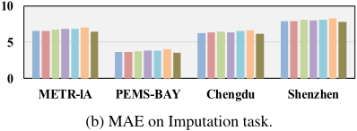
chosen different baselines for comparison. The proposed USTC surpasses all baselines across all metrics, indicating a more significant advantage than in the forecasting task. This superiority is attributed to that the imputation task is closer aligned with our pre-training, thus reducing the gap between pre-training and fine-tuning. Additionally, the imputation task is inherently more difficult due to the large missing data ratio we set, which explains the higher absolute MAE and RMSE values compared to those in the forecasting task.

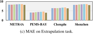
❸ Extrapolation. In the extrapolation task, we mask 30% of the nodes from the complete data, designating them as unobserved nodes. Our objective is to predict the future 1-hour data for these unobserved nodes using a 1-day historical dataset of the observed nodes. Similarly, we evaluate this task under two scenarios: transductive and inductive. In the transductive scenario, the model is trained on the full dataset with all nodes available. In the inductive scenario, the model is trained on incomplete data and does not have access to the masked nodes during training. The results are reported in Table 3. Also, we compare our method with exclusive baselines for the extrapolation task. The proposed USTC method surpasses all baselines across all metrics. This consistent outperformance across the three downstream tasks substantially validates the effectiveness of our framework.

Table 3: Imputation performance of transfer learning on the datasets. Trdu./Indu. denote transductive/inductive settings.

	Target City	METR-LA				PEMS-BAY				Chengdu				Shenzhen
Model	Metrics	MAE		RMSE		MAE		RMSE		MAE		RMSE		MAE		RMSE
	Setting	Trdu.	Indu.	Trdu.	Indu.	Trdu.	Indu.	Trdu.	Indu.	Trdu.	Indu.	Trdu.	Indu.	Trdu.	Indu.	Trdu.	Indu.
MEAN KNN	Target Only	10.28 9.11		14.86 12.88		5.49 4.2		9.28 7.55		7.42 7.01		9.78 9.4		8.81 8.89		11.08 11.17
KCN IGNNK	Reptile	5.64	7.75	8.70	11.75	3.89	4.72	6.86	8.19	6.60	7.00	8.95	9.28	5.68	8.25	8.04	10.94
		5.66	7.56	9.32	11.65	3.89	4.28	7.14	7.17	6.68	7.52	8.88	9.89	5.39	8.16	7.55	10.89
SATCN		4.80	7.49	7.83	11.57	3.45	3.84	6.49	6.79	6.57	7.09	9.00	9.39	5.50	8.11	7.86	10.82
DualSTN		5.59	7.09	9.57	11.45	3.53	3.71	6.80	6.74	5.94	6.37	8.05	8.66	5.34	8.17	7.61	10.89
INCREASE		4.99	7.34	8.22	11.49	3.41	3.68	6.38	6.77	6.13	6.62	8.49	8.78	5.33	8.14	7.60	10.82
STGP	Transfer	4.50	6.94	7.72	11.37	3.36	3.64	6.27	6.64	5.43	6.29	7.65	8.63	5.23	8.07	7.45	10.75
USTC	Transfer	4.29	6.46	7.26	11.21	3.27	3.55	6.20	6.58	4.99	6.17	7.49	8.48	5.15	7.82	7.35	10.47

Table 4: Extrapolation performance of transfer learning on the datasets. The results are averaged over all 12 future horizons.

	Target City	METR-LA				PEMS-BAY				Chengdu				Shenzhen
Model	Metrics	MAE		RMSE		MAE		RMSE		MAE		RMSE		MAE		RMSE
	Setting	Trdu.	Indu.	Trdu.	Indu.	Trdu.	Indu.	Trdu.	Indu.	Trdu.	Indu.	Trdu.	Indu.	Trdu.	Indu.	Trdu.	Indu.
MEAN	Target Only	10.64		15.27		5.56		9.31		7.53		9.74		8.91		11.63
GWN DCRNN IGNNK	Reptile	5.41	9.26	9.69	15.10	4.32	5.01	8.09	9.86	5.83	7.21	8.25	9.61	4.02	8.47	5.74	11.40
		5.10	9.41	9.19	15.57	3.64	5.12	6.97	10.14	6.23	7.10	8.62	9.58	3.85	8.64	5.31	11.54
		6.67	9.14	10.33	14.63	3.90	5.05	7.13	9.90	6.52	7.43	8.81	9.71	4.41	8.52	6.47	11.38
SATCN		7.29	9.13	12.41	14.88	4.65	5.13	9.04	10.13	7.09	7.20	9.51	9.66	4.87	8.70	7.15	11.58
ST-GFSL TPB TransGTR STGP	Transfer	7.73	9.31	12.31	14.99	4.27	4.59	7.61	7.92	6.51	6.79	8.74	9.41	4.75	8.55	6.99	11.45
		7.97	9.01	12.50	14.42	4.40	4.53	7.79	7.83	6.12	6.67	8.37	9.27	4.66	8.38	6.96	11.23
		7.33	8.87	11.22	14.12	4.55	4.66	7.95	8.10	6.42	6.62	8.65	9.10	4.58	8.45	6.81	11.36
		5.04	8.51	9.03	13.49	3.41	4.13	6.47	7.52	5.46	6.51	7.67	8.91	3.61	8.22	5.04	11.07
USTC	Transfer	4.82	8.19	8.94	13.21	3.18	3.99	6.17	7.28	5.26	6.33	7.48	8.74	3.44	8.09	4.96	10.82

4.3 Ablation Study

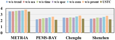
To deeply analyze the effect of different components in USTC, we design six variants of our model: 1) w/o trend, removing trend components from the framework; 2) w/o sea, removing seasonal components; 3) w/o time, removing time-domain signals; 4) w/o spec, removing frequency-domain signals; 5) w/o cons, removing the contrastive learning module from pretraining; 6) w/o prompt, removing the prompt module from fine-tuning. We report the MAE on the four datasets regarding all tasks of all variants and USTC in Fig. 4. As shown, the prompt module in fine-tuning state contributes a lot to our framework. The contrastive module in the pre-training stage has a contribution similar to but slightly less than the prompt module. Additionally, the involvement of both time- and frequency-domain signals results in ignorable performance improvement. Overall, all the proposed novel components have a positive impact on the improvement of our framework.

4.4 Impact of Pre-training Datasets

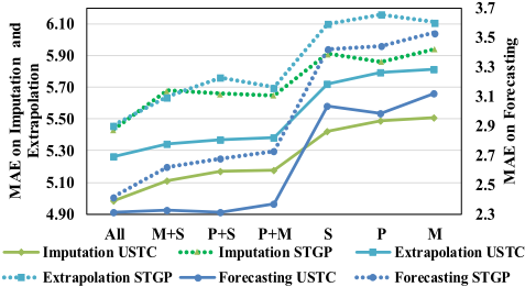
We further investigate the impact of varying pre-training datasets and assess the robustness of different methods. STGP is compared due to its significant performance. As shown in Fig. 3, when the number of source cities is reduced, the volume of training data correspondingly decreases, leading to a performance decline in both models. However, our USTC, which leverages several designed components in pre-training, experiences less degradation. This outcome underscores the robustness of USTC with limited data for pre-training.

5 Conclusion

In this paper, we propose a novel universal spatio-temporal modeling framework (USTC) generalized to various cities and tasks. To enhance the spatio-temporal representations during pre-training, we decouple the time-frequency patterns within the data and employ contrastive learning to preserve time-frequency consistency. Furthermore, we design a prompt generation module to extract personalized spatio-temporal patterns from the target city, which can be integrated with the learned common representations to collaboratively support downstream tasks. Extensive experiments validate the effectiveness of USTC in three downstream tasks across cities.

(a) MAE on Forecasting task.

Acknowledgments

This work was partly supported by the National Natural Science Foundation of China (Grant No.12227901) and the Project of Stable Support for Youth Team in Basic Research Field, Chinese Academy of Sciences (Grant No.YSBR-005).