
An End-to-End Simple Clustering Hierarchical Pooling Operation for Graph Learning Based on Top-K Node Selection
Proceedings of the Thirty-Fourth International Joint Conference on Artificial Intelligence. Main Track. Pages 3670-3679.
https://doi.org/10.24963/ijcai.2025/408
Keywords
- Data Mining: DM: Mining graphs
Abstract
Graph Neural Networks (GNNs) are powerful tools for graph learning, but one of the important challenges is how to effectively extract representations for graph-level tasks. In this paper, we propose an end-to-end Simple Clustering Hierarchical Pooling (SCHPool) operation, which is based on Top-K node selection for learning expressive graph representations. Specifically, SCHPool considers each node and its local neighborhood as a cluster, and introduces a novel multi-view scoring function to evaluate node importance. Based on these scores, clusters centered around the Top-K nodes are retained. This design eliminates the need for complex clustering operations, significantly reducing computational overhead. Furthermore, during the coarsening process, SCHPool employs a lightweight yet comprehensive attention mechanism to adaptively aggregate both the node features within clusters and the edge connectivity strengths between clusters. This facilitates the construction of more informative coarsened graphs, enhancing model performance. Experimental results demonstrate the effectiveness of the proposed model.
- [Baek et al., 2021] Jinheon Baek, Minki Kang, and Sung Ju Hwang. Accurate learning of graph representations with graph multiset pooling. In ICLR, 2021.
- [Bai et al., 2019] Lu Bai, Yuhang Jiao, Lixin Cui, and Ed- win R. Hancock. Learning aligned-spatial graph convolu- tional networks for graph classification. In ECML-PKDD, volume 11906, pages 464-482, 2019.
- [Bai et al., 2022a] Lu Bai, Lixin Cui, and Edwin R. Han- cock. A hierarchical transitive-aligned graph kernel for un-attributed graphs. In ICML, volume 162, pages 1327- 1336, 2022.
- [Bai et al., 2022b] Lu Bai, Lixin Cui, Yuhang Jiao, Luca Rossi, and Edwin R. Hancock. Learning backtrackless aligned-spatial graph convolutional networks for graph classification. IEEE Transactions on Pattern Analysis and Machine Intelligence, 44(2):783-798, 2022.
- [Bai et al., 2023] Lu Bai, Yuhang Jiao, Lixin Cui, Luca Rossi, Yue Wang, Philip S. Yu, and Edwin R. Hancock. Learning graph convolutional networks based on quan- tum vertex information propagation. IEEE Transactions on Knowledge and Data Engineering, 35(2):1747-1760, 2023.
- [Bai et al., 2024] Lu Bai, Lixin Cui, Yue Wang, Ming Li, Jing Li, Philip S. Yu, and Edwin R. Hancock. HAQJSK: hierarchical-aligned quantum jensen-shannon kernels for graph classification. IEEE Transactions on Knowledge and Data Engineering, 36(11):6370-6384, 2024.
- [Bianchi and Lachi, 2023] Filippo Maria Bianchi and Veron- ica Lachi. The expressive power of pooling in graph neural networks. In NeurIPS, pages 71603-71618, 2023.
- [Bianchi et al., 2020] Filippo Maria Bianchi, Daniele Grat- tarola, and Cesare Alippi. Spectral clustering with graph neural networks for graph pooling. In ICML, volume 119, pages 874-883, 2020.
- [Borgwardt et al., 2005] Karsten M. Borgwardt, Cheng Soon Ong, Stefan Schönauer, S. V. N. Vishwanathan, Alexan- der J. Smola, and Hans-Peter Kriegel. Protein function prediction via graph kernels. In ISMB, pages 47-56, 2005.
- [Chen et al., 2019] Hongxu Chen, Hongzhi Yin, Tong Chen, Quoc Viet Hung Nguyen, Wen-Chih Peng, and Xue Li. Exploiting centrality information with graph convolutions for network representation learning. In ICDE, pages 590- 601, 2019.
- [Cui et al., 2024] Lixin Cui, Lu Bai, Xiao Bai, Yue Wang, and Edwin R. Hancock. Learning aligned vertex con- volutional networks for graph classification. IEEE Transactions on Neural Networks and Learning Systems, 35(4):4423-4437, 2024.
- [Dobson and Doig, 2003] Paul D Dobson and Andrew J Doig. Distinguishing enzyme structures from non- enzymes without alignments. Journal of molecular biol- ogy, 330(4):771-783, 2003.
- [Duvenaud et al., 2015] David Duvenaud, Dougal Maclau- rin, Jorge Aguilera-Iparraguirre, Rafael Gómez- Bombarelli, Timothy Hirzel, Alán Aspuru-Guzik, and Ryan P. Adams. Convolutional networks on graphs for learning molecular fingerprints. In NeurIPS, pages 2224-2232, 2015.
- [Errica et al., 2020] Federico Errica, Marco Podda, Davide Bacciu, and Alessio Micheli. A fair comparison of graph neural networks for graph classification. In ICLR, 2020.
- [Gao and Ji, 2019] Hongyang Gao and Shuiwang Ji. Graph u-nets. In ICML, volume 97, pages 2083-2092, 2019.
- [Gao et al., 2021] Hongyang Gao, Yi Liu, and Shuiwang Ji. Topology-aware graph pooling networks. IEEE Trans- actions on Pattern Analysis and Machine Intelligence, 43(12):4512-4518, 2021.
- [Gao et al., 2022] Xing Gao, Wenrui Dai, Chenglin Li, Hongkai Xiong, and Pascal Frossard. ipool -information- based pooling in hierarchical graph neural networks. IEEE Transactions on Neural Networks and Learning Systems, 33(9):5032-5044, 2022.
- [Hochreiter and Schmidhuber, 1997] Sepp Hochreiter and Jürgen Schmidhuber. Long short-term memory. Neural Computation, 9(8):1735-1780, 1997.
- [Ju et al., 2024] Wei Ju, Zheng Fang, Yiyang Gu, Zequn Liu, Qingqing Long, Ziyue Qiao, Yifang Qin, Jianhao Shen, Fang Sun, Zhiping Xiao, Junwei Yang, Jingyang Yuan, Yusheng Zhao, Yifan Wang, Xiao Luo, and Ming Zhang. A comprehensive survey on deep graph representation learning. Neural Networks, 173:106207, 2024.
- [Knyazev et al., 2019] Boris Knyazev, Graham W. Taylor, and Mohamed R. Amer. Understanding attention and gen- eralization in graph neural networks. In NeurIPS, pages 4204-4214, 2019.
- [Lee et al., 2019] Junhyun Lee, Inyeop Lee, and Jaewoo Kang. Self-attention graph pooling. In ICML, volume 97, pages 3734-3743, 2019.
- [Li et al., 2016] Yujia Li, Daniel Tarlow, Marc Brockschmidt, and Richard S. Zemel. Gated graph sequence neural networks. In ICLR, 2016.
- [Li et al., 2018] Yaguang Li, Rose Yu, Cyrus Shahabi, and Yan Liu. Diffusion convolutional recurrent neural net- work: Data-driven traffic forecasting. In ICLR, 2018.
- [Liu et al., 2022] Yue Liu, Lixin Cui, Yue Wang, and Lu Bai. Abdpool: Attention-based differentiable pooling. In ICPR, pages 3021-3026, 2022.
- [Liu et al., 2023a] Chuang Liu, Yibing Zhan, Jia Wu, Chang Li, Bo Du, Wenbin Hu, Tongliang Liu, and Dacheng Tao. Graph pooling for graph neural networks: Progress, chal- lenges, and opportunities. In IJCAI, pages 6712-6722, 2023. IJCAI
- [Liu et al., 2023b] Chuang Liu, Yibing Zhan, Baosheng Yu, Liu Liu, Bo Du, Wenbin Hu, and Tongliang Liu. On exploring node-feature and graph-structure diversities for node drop graph pooling. Neural Networks, 167:559-571, 2023.
- [Orsini et al., 2015] Francesco Orsini, Paolo Frasconi, and Luc De Raedt. Graph invariant kernels. In IJCAI, pages 3756-3762, 2015.
- [Qu et al., 2017] Meng Qu, Jian Tang, Jingbo Shang, Xiang Ren, Ming Zhang, and Jiawei Han. An attention-based collaboration framework for multi-view network represen- tation learning. In CIKM, pages 1767-1776, 2017.
- [Ranjan et al., 2020] Ekagra Ranjan, Soumya Sanyal, and Partha P. Talukdar. ASAP: adaptive structure aware pool- ing for learning hierarchical graph representations. In AAAI, pages 5470-5477, 2020.
- [Schlichtkrull et al., 2018] Michael Sejr Schlichtkrull, Thomas N. Kipf, Peter Bloem, Rianne van den Berg, Ivan Titov, and Max Welling. Modeling relational data with graph convolutional networks. In ESWC, volume 10843, pages 593-607, 2018.
- [Shervashidze et al., 2011] Nino Shervashidze, Pascal Schweitzer, Erik Jan van Leeuwen, Kurt Mehlhorn, and Karsten M. Borgwardt. Weisfeiler-lehman graph kernels. Journal of Machine Learning Research, 12:2539-2561, 2011.
- [Sun et al., 2020] Mengying Sun, Sendong Zhao, Coryan- dar Gilvary, Olivier Elemento, Jiayu Zhou, and Fei Wang. Graph convolutional networks for computational drug de- velopment and discovery. Briefings in Bioinformatics, 21(3):919-935, 2020.
- [Vinyals et al., 2016] Oriol Vinyals, Samy Bengio, and Man- junath Kudlur. Order matters: Sequence to sequence for sets. In ICLR, 2016.
- [Wale et al., 2008] Nikil Wale, Ian A. Watson, and George Karypis. Comparison of descriptor spaces for chemical compound retrieval and classification. Knowledge and In- formation Systems, 14(3):347-375, 2008.
- [Wu et al., 2022] Junran Wu, Xueyuan Chen, Ke Xu, and Shangzhe Li. Structural entropy guided graph hierarchi- cal pooling. In ICML, volume 162, pages 24017-24030, 2022.
- [Wu et al., 2023] Shiwen Wu, Fei Sun, Wentao Zhang, Xu Xie, and Bin Cui. Graph neural networks in recom- mender systems: A survey. ACM Computing Surveys, 55(5):97:1-97:37, 2023.
- [Xu et al., 2019] Keyulu Xu, Weihua Hu, Jure Leskovec, and Stefanie Jegelka. How powerful are graph neural net- works? In ICLR, 2019.
- [Yanardag and Vishwanathan, 2015] Pinar Yanardag and S. V. N. Vishwanathan. Deep graph kernels. In SIGKDD, pages 1365-1374, 2015.
- [Ye et al., 2023] Rongji Ye, Lixin Cui, Luca Rossi, Yue Wang, Zhuo Xu, Lu Bai, and Edwin R. Hancock. C2N-ABDP: cluster-to-node attention-based differen- tiable pooling. In GbRPR, volume 14121, pages 70-80, 2023.
- [Ying et al., 2018] Zhitao Ying, Jiaxuan You, Christopher Morris, Xiang Ren, William L. Hamilton, and Jure Leskovec. Hierarchical graph representation learning with differentiable pooling. In NeurIPS, pages 4805-4815, 2018.
- [Yuan and Ji, 2020] Hao Yuan and Shuiwang Ji. Structpool: Structured graph pooling via conditional random fields. In ICLR, 2020.
- [Zhang et al., 2018] Muhan Zhang, Zhicheng Cui, Marion Neumann, and Yixin Chen. An end-to-end deep learn- ing architecture for graph classification. In AAAI, pages 4438-4445, 2018.
- [Zhang et al., 2023] Zhen Zhang, Jiajun Bu, Martin Ester, Jianfeng Zhang, Zhao Li, Chengwei Yao, Huifen Dai, Zhi Yu, and Can Wang. Hierarchical multi-view graph pooling with structure learning. IEEE Transactions on Knowledge and Data Engineering, 35(1):545-559, 2023.
References were extracted automatically from the PDF and may contain errors.
Full text extracted automatically from the PDF; figures, tables and equations may differ. The PDF is the version of record.
1 Introduction
Graph-structured data, such as social networks and molecular structures, are prevalent in the real world. Some researchers have employed graph kernel methods to process such data by computing pairwise similarities between graphs [Shervashidze et al., 2011; Bai et al., 2022a; Bai et al., 2024]. However, these methods typically lack support for end-to-end training and incur high computational costs, making them difficult to scale to large graphs. With the continued advancement of deep learning techniques, Graph Neural Networks
∗Corresponding Authors: Lu Bai and Hangyuan Du
(GNNs) have emerged as powerful tools for effectively processing such non-Euclidean data. By simultaneously capturing node features and complex topological relationships between nodes, GNNs are able to generate meaningful lowdimensional representations. This capability has led to their widespread application in various fields, including knowledge graphs [Schlichtkrull et al., 2018], recommendation systems [Wu et al., 2023], traffic prediction [Li et al., 2018], and drug discovery [Sun et al., 2020].
One challenge arising in GNNs is to extract meaningful representations for graph-level tasks [Bai et al., 2022b], such as graph classification [Errica et al., 2020] and graph regression [Bianchi et al., 2020]. To address this issue, various graph pooling methods have been proposed, which can generally be categorized into global pooling and hierarchical pooling [Ju et al., 2024]. Global pooling [Bai et al., 2019; Cui et al., 2024], similar to pooling operations in traditional neural networks, applies a function to all node embeddings to produce a graph-level representation. However, such methods overlook the hierarchical characteristics inherent in graphs.
To overcome this shortcoming, researchers have proposed hierarchical pooling operations, which extract hierarchical characteristics of a graph by progressively compressing it. Based on the compression method, hierarchical pooling operations can be broadly divided into two categories, i.e., the Top-K based strategy and the cluster-based strategy.
The Top-K based strategy employs scoring functions to assess the importance of nodes, retaining the Top-K nodes and their corresponding connections as the coarsened graph. However, most existing methods rely on single-view evaluations, which are prone to bias [Qu et al., 2017; Chen et al., 2019]. Furthermore, information from different views often varies significantly, making it crucial to leverage the collaboration of multiple views to learn robust node importance scores. Although some multi-view methods have been introduced [Zhang et al., 2023], they are limited by inherent drawbacks of the Top-K based strategy. Specifically, direct removal of nodes and edges in such methods often results in a substantial loss of node information, impairing the connectivity of the coarsened graph [Ju et al., 2024].
On the other hand, the cluster-based strategy assigns nodes to different clusters using learnable assignment matrices [Liu et al., 2023a], treating these clusters as nodes in the coarsened graph. Although this strategy preserves all node and edge information, it is subject to several inherent limitations. First, these methods are constrained by both time and memory complexity, primarily due to the need for complex and dense assignment matrices, which typically incurs O(N 2 ) complexity [Baek et al., 2021]. Second, in some approaches, node features are probabilistically divided into different clusters and then directly summed to form cluster representations. This assignment strategy can lead to influential nodes being split across multiple clusters, while less influential nodes are assigned entirely to a single cluster, potentially resulting in the latter dominating the cluster representations. Although some studies have attempted to address this issue by completely assigning nodes to clusters and applying attention-based aggregation, they fail to provide a comprehensive evaluation of node importance [Liu et al., 2022]. Third, when performing convolution on the coarsened graphs, edge connectivity strengths can naturally serve as attention weights, guiding selective neighborhood information aggregation. However, previous methods typically aggregate edge connectivity strengths between clusters via simple summation, without considering the importance of edge. This leads to aggregated edge connectivity strengths that fail to accurately reflect the influence of information propagation between clusters.
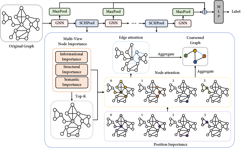
To address the aforementioned limitations, we propose an end-to-end Simple Clustering Hierarchical Pooling (SCHPool) operation based on Top-K node selection. Unlike previous cluster-based methods that rely on the computation of complex and dense assignment matrices, SCHPool introduces an innovative approach by directly treating each node and its local neighborhood as a cluster. A multi-view scoring function is then employed to assess node importance from informational, structural, and semantic perspectives, and clusters centered around the Top-K nodes are subsequently retained. During the coarsening process, we employ a lightweight yet comprehensive attention mechanism to adaptively aggregate node features within clusters. This mechanism considers not only the multi-view importance of each node, but also its relative position within the cluster. Moreover, the aggregation weights of edges are computed based on the attention weights of their connected nodes within the corresponding clusters. The architecture of the proposed SCHPool is illustrated in Figure 1, and main contributions are summarized as follows.
First, compared to the Top-K based strategy, SCHPool preserves richer node and edge information. Moreover, SCHPool introduces a novel multi-view scoring function, even when the model degenerates into the Top-K based strategy, it still outperforms existing Top-K based methods. Second, compared to the cluster-based strategy, SCHPool eliminates the need for computing complex and dense assignment matrices, reducing the complexity to O(E +N). Moreover, it incorporates a lightweight yet comprehensive attention mechanism to adaptively aggregate both node features within clusters and edge connectivity strengths between clusters, leading to more informative coarsened graphs. Third, we evaluated the classification performance of the SCHPool, experimental results demonstrate its effectiveness.
2 RelatedWorks
2.1 The Global Pooling
Global pooling operations directly generate a graph representation from all node embeddings [Bai et al., 2023], which are also known as readout functions. The foundational global pooling methods are inspired by traditional pooling operations in Convolutional Neural Networks (CNNs), such as Max-Pooling, Sum-Pooling, and Mean-Pooling, which apply permutation-invariant functions to node embeddings in a graph [Duvenaud et al., 2015; Xu et al., 2019]. Set2Set [Vinyals et al., 2016] implements global pooling by aggregating node information through LSTMs [Hochreiter and Schmidhuber, 1997]. To further enhance adaptability, GGSNN [Li et al., 2016] incorporates a soft attention mechanism to assess node importance, computing the weighted sum of node embeddings to form the graph representation. SortPool [Zhang et al., 2018], on the other hand, ranks nodes based on their structural positions within the graph, generating the graph representation by processing the ordered node embeddings through CNNs. More recently, GMT [Baek et al., 2021] captures node interactions through a multi-head attention mechanism, further improving the performance of global pooling methods. However, these operations fail to account for the hierarchical structures of graphs, which can result in information loss and impair the performance of graph representations [Knyazev et al., 2019; Bianchi and Lachi, 2023].
2.2 The Hierarchical Pooling
Hierarchical pooling methods capture the hierarchical structure of a graph by progressively coarsening it, which are achieved through the Top-K based strategy and the clusterbased strategy. Furthermore, it is important to note that these methods still rely on readout functions to obtain the graph representation from coarsened graphs.
The Top-K based strategy involves learning the importance values of nodes and retaining the Top-K nodes and their connections as the coarsened graph. Different methods employ various approaches to assess node importance. Some methods predict from a single view, such as scalar projection values in TopKPool [Gao and Ji, 2019] and self-attention weights in SAGPool [Lee et al., 2019]. Other methods, such as TAPool [Gao et al., 2021] and MVPool [Zhang et al., 2023], generate scores from multiple views for a comprehensive evaluation. Although these methods are efficient, they suffer from inevitable information loss [Liu et al., 2023b].
The cluster-based strategy clusters the nodes and aggregates them to form the coarsened graph. Existing operations primarily focus on optimizing the clustering procedure. For example, DiffPool [Ying et al., 2018] employs GNNs to generate assignment matrices. StructPool [Yuan and Ji, 2020] utilizes conditional random fields to capture the relationships among the assignments of different nodes, determining each node's assignment based on its own features and the assignments of other nodes. MinCutPool [Bianchi et al., 2020] leverages spectral clustering to group nodes, and SEP-G [Wu et al., 2022] minimizes structural entropy to construct a coding tree from nodes to achieve effective hierarchical pooling.
However, these methods aggregate node features within clusters merely through simply summation. To overcome this limitation, ABDPool [Liu et al., 2022] and C2N-ABDP [Ye et al., 2023] incorporate attention mechanisms into the aggregation process. Nevertheless, these attention mechanisms suffer from two key limitations. First, they rely on a single perspective, restricting their ability to comprehensively evaluate node importance. Second, they are incapable of capturing the importance of edges. Furthermore, although these cluster-based methods preserve the information of graphs completely, they often suffer from low computational efficiency, which restricts their scalability to large-scale graphs.
3 The ProposedMethod
3.1 Preliminaries
We represent the input graph as G(0) (V (0) ,E(0) ), where V denotes the nodes and E denotes the edges. Since hierarchical pooling operations change the number of nodes and edges at each pooling layer, we define the graph at the lth layer as G(l) (V (l) ,E(l) ). The connectivity strengths between nodes of G(l) can be represented by an adjacency matrix A(l) ∈ RNl×Nl , where Nl = |V (l) | is the number of nodes at the l-th layer. X(l) ∈ RNl×dl represents the node feature matrix, where dl is the feature dimension at l-th layer. Moreover, we employ a Graph Neural Network (GNN) to obtain the node embeddings matrix Z (l) ∈ RNl×dl ′ as
3.2 The Multi-ViewNode Importance
The Informational Importance. Informational nodes play a crucial role in characterizing graph signals. If a node's information can be effectively predicted given the information of its neighbors, it indicates that the node carries less unique information, and therefore has a lower importance. We propose to leverage the neighborhood conditional entropy as a metric for assessing the informational importance of nodes as
where z(l) i represents the embedding of node i at l-th layer, and N(i) denotes the set of its neighboring nodes. H(·) denotes entropy, and I(·) represents mutual information.
To simplify the computation, inspired by iPool [Gao et al., 2022], we use neighborhood information gain as an approximate empirical estimation of H(z(l) i |z(l) N(i) ) (proved in the Appendix A). We define the neighborhood information gain γ as the Euclidean distance between a node embedding and the embedding predicted by its neighbors, i.e.,
Considering the localization and smoothness properties of graphs, we use a simple neighborhood normalization aggregation function as the prediction function f(·). The normalization process is defined as
where ¯ A(l) is the adjacency matrix with all self-loops removed from A(l) , and ¯ D(l) is the corresponding degree matrix. Based on this, the prediction function f(·) performs neighborhood aggregation as
Moreover, we apply a non-linear activation function σ(·) to transform the values into range [0, 1], i.e.,
The Structural Importance. We identify structurally critical nodes in the graph based on their local connectivity. Nodes embedded in denser and more stable local connections are considered to play more significant roles within the graph. Moreover, since SCHPool naturally treats each node and its neighborhood as a cluster, this approach also implicitly identifies important clusters, thereby increasing their likelihood of being retained during pooling. To quantify this, we adopt two perspectives, summation and variance, to characterize the distribution of edge connectivity strengths within a node's local neighborhood, i.e., the cluster centered around it. Specifically, we first construct a mask matrix B(l) ∈ RNl×Nl , i.e.,
where B(l) ij indicates whether node j belongs to the cluster centered around node i (hereafter referred to as cluster i), and H is a hyperparameter that represents the clustering range.
Next, we calculate the degree matrix R(l) ∈ RNl×Nl as
And it is important to note that the degree here only counts connections between nodes within the same cluster. Consequently, the total sum of edge connectivity strengths between nodes within cluster i can be computed as
Since directly calculating the variance of edge connectivity strengths within a cluster is computationally expensive, we approximate it using the variance of node degrees within the cluster. Specifically, the number of nodes in cluster i is
and the mean degree of nodes within the cluster i is
Then, the degree variance within the cluster i is calculated as
Consequently, the structural importance can be computed as
The Semantic Importance. The semantic importance of a node reflects the degree to which its embedding contributes meaningful information to downstream tasks. To assess this, inspired by SAGPool [Lee et al., 2019], we adopt a learnable module (e.g., a multi-layer perceptron (MLP)) that assigns self-attention weights to nodes in an end-to-end manner. This enables the model to focus on the most discriminative nodes within the graph. The semantic importance is computed as
The Multi-View Node Importance. These three perspectives-informational, structural, and semantic-are complementary, each capturing a distinct aspect of node importance. To facilitate their collaboration in generating more comprehensive and robust node importance scores, we introduce three normalized trainable parameters (i.e., δ(l) x +δ(l) y +δ(l) z = 1), which serve as weights for each view. The final multi-view node importance score is computed as
3.3 The AttentionMechanism
To construct more informative coarsened graphs, it is essential to aggregate node features within each cluster based on their importance, thereby generating more expressive cluster representations. Although we introduced the multi-view node importance score (in Section 3.2), a global metric for assessing node importance that remains consistent across all clusters, it is not sufficiently comprehensive. Relying solely on this score as the attention weight for node aggregation may cause a highly important node to dominate the information in its surrounding clusters, resulting in overly similar representations among neighboring clusters.
To address this issue, we introduce a new metric to assist in evaluating node importance based on its structural role within the corresponding cluster. Since our method forms clusters around center nodes, we assign an importance weight to each node according to its relative position within the cluster, i.e., its distance from the center node. This Position Importance is then combined with the multi-view node importance to determine the final attention weight of each node within the corresponding cluster. As a result, the attention weight of the same node may vary across different clusters.
Specifically, for each distance h, we normalize the multiview importance scores of nodes that are h hops away from the cluster center node j, which is defined as
Then, we learn different position importance parameters ϕ(l) h for nodes at varying distances from the center, and combine them with the normalized multi-view node importance scores to derive the node attention matrix M (l) ∈ RNl×Nl as
where ∑Hh=0 ϕ(l) h = 1, and H is a hyperparameter that represents the clustering range. M (l) ij indicates the attentionweight of node i within the cluster centered at node j.
3.4 The Graph Pooling
To coarsen the graph at the l-th layer, we first extract the indices of the Top-K nodes based on the multi-view node importance scores ω(l) as
where Nl+1 = ⌈kNl⌉ represents the number of nodes in the (l + 1)-th layer and k is the pooling ratio.
We then directly extract the corresponding columns from the node attention matrix M (l) ∈ RNl×Nl using these indices to construct the assignment matrix S(l) ∈ RNl×Nl+1 as
This operation eliminates the need for additional computational resources to learn assignment matrices, while directly providing the attention weights for nodes within each cluster.
Then, we use this assignment matrix to perform node attention aggregation within each cluster, obtaining the node feature matrix X(l+1) ∈ RNl+1×dl ′ in the next layer as
Since our approach allows a single node to belong to multiple clusters, the same edge may be associated with different cluster pairs during edge aggregation. Therefore, the attention coefficient for an edge should vary depending on the clusters to which it connects. To simplify the computation, we compute the attention weight for an edge as the product of attention weights of the connected nodes within their respective clusters. In other words, we assume that the connections between more important nodes are more significant. Thus, the edge connectivity strength between clusters p and q in the next layer can be computed as
and the weighted aggregation adjacency matrix A(l+1) ∈ RNl+1×Nl+1 for the coarsened graph can be computed as
| Method | Assignment Matrix | Computational Complexity ① |
|---|---|---|
| DiffPool | S = softmax(GNN(X,A)) | O(KN 2 ) |
| StructPool | S : Minimize E(S) ② | O(N 3 ) |
| MinCutPool | S =MLP(X) , minCUT loss ③ | O((E + NK)K) |
| SEP-G | S : Minimize HT (G) ④ | O(2N + logN(E logN +N)) |
| ABDPool | S = argmax(GNN(X,A)) | O(KN 2 )⑤ |
| SCHPool | S = M(:, idx)⑥ | O(E + N) |
- ① N and E denote the number of nodes and edges respectively, and K denotes the number of nodes after pooling.
- ② E(·) is the Gibbs energy, including unary energy and pairwise energy.
- ③ minCUT loss consists of cut loss, which approximates the mincut problem, and orthogonality loss, which spurs the assignments to be orthogonal.
- ④ HT (G) is the structural entropy for G on coding tree T .
- ⑤ Note that the complexity analysis is based on processing a single graph. Although ABDPool and DiffPool have equivalent theoretical complexities, ABDPool computes node attention through iterative processing of each graph, which prevents parallelization. As a result, its practical computational efficiency is significantly lower than that of DiffPool.
- ⑥ M denotes the node attention matrix, as defined in Eq. (17).
Table 1: Comparison of SCHPool and Other Cluster-based Methods.
3.5 The Computational Complexity
Unlike previous cluster-based hierarchical pooling methods (as summarized in Table 1), both the adjacency and assignment matrices of the SCHPool can be stored and computed using sparse tensors, reducing the computational complexity to O(E + N). More specifically, the complexity of GNN operation is O(EF + NFF ′ ) ≈ O(E + N), where the feature dimensions F and F ′ are constants. The computation of informational importance involves operations of complexity O(EF ′ ) ≈ O(E), while semantic importance requires only O(NF ′ ) ≈ O(N). Structural importance involves multiplying two sparse matrices, with complexity O(E · dB), where dB is the average number of non-zero elements per column in matrix B. Since dB is typically small and bounded, the complexity can be approximated as O(E). During the pooling stage, no additional computations are needed for the sparse assignment matrix S. Node aggregation exhibits a complexity of O(ESF ′ ) ≈ O(ES), where ES < E. Edge aggregation involves two sparse matrix multiplications and thus shares the same complexity as the structural importance computation, i.e., approximately O(E). In summary, the overall computational complexity of SCHPool is O(E +N).
4 Experiments
We empirically evaluate the proposed method against other deep learning approaches for graph classification on nine benchmarks, including D&D [Dobson and Doig, 2003], PROTEINS [Borgwardt et al., 2005], NCI1, NCI109 [Wale et al., 2008], FRANKENSTEIN [Orsini et al., 2015], IMDB-B, IMDB-M, COLLAB, and REDDIT-B [Yanardag and Vishwanathan, 2015]. Detailed statistics are shown in the Table 2. Note that when nodes in a graph lack labels or features, the node degree can be used as the label.
4.1 Baselines and Experimental Settings
We adopt eight hierarchical pooling methods as baselines for comparison, which include three Top-K based methods: SAGPool(H) [Lee et al., 2019], TopKPool [Gao and Ji, 2019], and ASAP [Ranjan et al., 2020], as well as five cluster-based methods: DiffPool [Ying et al., 2018], StructPool [Yuan and Ji, 2020], MinCutPool [Bianchi et al., 2020], SEP-G [Wu et al., 2022], and ABDPool [Liu et al., 2022]. Moreover, we consider four global pooling methods for comparison: Set2Set [Vinyals et al., 2016], SortPool [Zhang et al., 2018], SAGPool(G) [Lee et al., 2019], and GMT [Baek et al., 2021].
| Dataset | Graphs | Classes | Vertices(Avg.) | Edges(Avg.) | Edge Density(Avg.) | Clustering coefficient(Avg.) | Labels/Attributes | Domain |
|---|---|---|---|---|---|---|---|---|
| D&D | 1178 | 2 | 284.32 | 715.66 | 0.028 | 0.480 | Labels | Biochemical |
| PROTEINS | 1113 | 2 | 39.06 | 72.82 | 0.212 | 0.513 | Labels | Biochemical |
| NCI1 | 4110 | 2 | 29.87 | 32.30 | 0.089 | 0.003 | Labels | Biochemical |
| NCI109 | 4127 | 2 | 29.68 | 32.13 | 0.089 | 0.003 | Labels | Biochemical |
| FRANKENSTEIN | 4337 | 2 | 16.90 | 17.88 | 0.171 | 0.011 | Attributes | Biochemical |
| IMDB-B | 1000 | 2 | 19.77 | 96.53 | 0.521 | 0.947 | - | Social |
| IMDB-M | 1500 | 3 | 13.00 | 65.94 | 0.772 | 0.969 | - | Social |
| COLLAB | 5000 | 3 | 74.49 | 2457.78 | 0.509 | 0.891 | - | Social |
| REDDIT-B | 2000 | 2 | 429.63 | 497.75 | 0.022 | 0.059 | - | Social |
| D&D | PROTEINS | NCI1 | NCI109 | FRANKENSTEIN | IMDB-B | IMDB-M | COLLAB | REDDIT-B | |
|---|---|---|---|---|---|---|---|---|---|
| Set2Set | 71.94 ± 0.56 | 73.27 ± 0.85 | 68.55 ± 1.92 | 61.04 ± 2.69 | 61.46 ± 0.47 | 72.90 ± 0.75 | 50.19 ± 0.39 | 79.55 ± 0.39 | - |
| SortPool | 75.58 ± 0.72 | 73.17 ± 0.88 | 73.82 ± 1.96 | 68.59 ± 0.67 | 63.44 ± 0.65 | 72.12 ± 1.12 | 48.18 ± 0.83 | 77.87 ± 0.47 | 76.02 ± 1.73 |
| SAGPool(G) | 71.54 ± 0.91 | 72.02 ± 1.08 | 74.18 ± 1.20 | 74.06 ± 0.78 | 62.57 ± 0.60 | 72.16 ± 0.88 | 49.47 ± 0.56 | 78.85 ± 0.56 | 74.45 ± 1.73 |
| GMT | 78.72 ± 0.59 | 75.09 ± 0.59 | 76.35 ± 2.62 | 74.87 ± 0.47 | 62.69 ± 0.25 | 73.48 ± 0.76 | 50.66 ± 0.82 | 80.74 ± 0.54 | - |
| SAGPool(H) | 74.72 ± 0.82 | 71.56 ± 1.49 | 67.45 ± 1.11 | 67.86 ± 1.41 | 61.73 ± 0.76 | 72.55 ± 1.28 | 50.23 ± 0.44 | 78.03 ± 0.31 | 75.53 ± 3.53 |
| TopKPool | 73.63 ± 0.55 | 70.48 ± 1.01 | 67.02 ± 2.25 | 66.12 ± 1.60 | 61.46 ± 0.84 | 71.58 ± 0.95 | 48.59 ± 0.72 | 77.58 ± 0.85 | 85.12 ± 0.34 |
| ASAP | 76.58 ± 1.04 | 73.92 ± 0.63 | 71.48 ± 0.42 | 70.07 ± 0.55 | 66.26 ± 0.47 | 72.81 ± 0.50 | 50.78 ± 0.75 | 78.64 ± 0.50 | - |
| DiffPool | 77.56 ± 0.41 | 73.03 ± 1.00 | 62.32 ± 1.90 | 61.98 ± 1.98 | 60.60 ± 1.62 | 73.14 ± 0.70 | 51.31 ± 0.72 | 78.68 ± 0.43 | 82.12 ± 1.06 |
| StructPool | 78.45 ± 0.40 | 75.16 ± 0.86 | 78.64 ± 1.53 | - | - | 72.06 ± 0.64 | 50.23 ± 0.53 | 77.27 ± 0.51 | - |
| MinCutPool | 78.22 ± 0.54 | 74.72 ± 0.48 | 74.25 ± 0.86 | 74.05 ± 2.48 | 61.65 ± 0.72 | 72.65 ± 0.75 | 51.04 ± 0.70 | 80.87 ± 0.34 | - |
| SEP-G | 77.98 ± 0.57 | 76.42 ± 0.39 | 78.35 ± 0.33 | 73.17 ± 0.42 | - | 74.12 ± 0.56 | 51.53 ± 0.65 | 81.28 ± 0.15 | - |
| ABDPool | 74.13 ± 0.52 | 73.24 ± 0.91 | 71.54 ± 1.28 | 71.78 ± 1.35 | - | 70.58 ± 0.71 | 50.63 ± 1.47 | - | 82.75 ± 0.82 |
| SCHPool | 78.79 ± 0.31 | 77.09 ± 0.13 | 77.22 ± 0.11 | 75.91 ± 0.20 | 69.53 ± 0.20 | 74.45 ± 0.28 | 53.02 ± 0.15 | 81.96 ± 0.08 | 85.82 ± 0.24 |
| Hyperparameter | Range |
|---|---|
| Learning rate Pooling ratio Pooling layer Clustering range | 5e-3, 1e-3, 5e-4 0.25, 0.5, 0.8 1, 2, 3, 4 1, 2 |
In our experiments, we employ 10-fold cross-validation for evaluation and report the average accuracy along with the standard deviation over 10 runs. For the proposed SCHPool, we utilize a 3-layer GNN model with an output dimension of 64 to generate node embeddings. Furthermore, we perform hyperparameter tuning using a grid search strategy (as detailed in the Table 4). Our code is publicly available. 1
4.2 Results and Discussions
Table 3 shows that the proposed SCHPool outperforms all alternative methods on eight of the nine datasets, particularly the FRANKENSTEIN dataset, indicating that our method excels on datasets with node attributes. The only exception is the NCI1 dataset, where the accuracy of two cluster-based hierarchical pooling methods, StructPool and SEP-G, is slightly higher than that of SCHPool. The effectiveness of SCHPool can be attributed to three key factors.
1 https://github.com/zhzhaoo/SCHPool
| PROTEINS | FRANKENSTEIN | IMDB-M | |
|---|---|---|---|
| Top-K based | 76.38 ± 0.16 | 67.94 ± 0.31 | 52.77 ± 0.18 |
| Cluster based | 77.09 ± 0.13 | 69.53 ± 0.20 | 53.02 ± 0.15 |
First, unlike global pooling methods, SCHPool is able to capture hierarchical structural characteristics of the graph, resulting in a more refined graph representation. Second, compared to Top-K based pooling methods, SCHPool preserves more node information and generates coarsened graphs with better connectivity. Furthermore, SCHPool introduces an effective multi-view scoring function to evaluate node importance. Even when the model degenerates into the TopK based strategy, it still outperforms existing Top-K based methods (as shown in Table 5). Third, in contrast to previous cluster-based pooling methods, SCHPool integrates a comprehensive attention mechanism to adaptively aggregate node features within clusters and edge connectivity strengths between clusters. This enables the construction of more informative coarsened graphs, enhancing the model performance. Thus, the proposed SCHPool model outperforms previous methods on most datasets.
4.3 The Ablation Study
To further evaluate the effectiveness of each component in the proposed SCHPool, we perform ablation experiments on three representative datasets: PROTEINS (from the biochemical domain with node labels), FRANKENSTEIN (from the biochemical domain with node attributes), and IMDB-M (from the social domain without node labels and attributes).
| PROTEINS | FRANKENSTEIN | IMDB-M | |
|---|---|---|---|
| Informational | 76.63 ± 0.20 | 68.66 ± 0.31 | 52.85 ± 0.07 |
| Structural | 75.89 ± 0.36 | 68.65 ± 0.18 | 52.31 ± 0.24 |
| Semantic | 75.67 ± 0.11 | 68.73 ± 0.16 | 52.75 ± 0.24 |
| w/o Informational | 76.17 ± 0.09 | 68.99 ± 0.21 | 52.78 ± 0.17 |
| w/o Structural | 76.42 ± 0.25 | 68.59 ± 0.13 | 52.83 ± 0.16 |
| w/o Semantic | 76.67 ± 0.24 | 69.39 ± 0.23 | 52.87 ± 0.12 |
| Multi-View | 77.09 ± 0.13 | 69.53 ± 0.20 | 53.02 ± 0.15 |
| PROTEINS | FRANKENSTEIN | IMDB-M | |
|---|---|---|---|
| w/o Att. Mech. | 75.78 ± 0.59 | 68.96 ± 0.23 | 52.21 ± 0.13 |
| Att. Mech. (w/o Pos.) | 76.50 ± 0.30 | 68.77 ± 0.13 | 52.81 ± 0.19 |
| AttentionMechanism | 77.09 ± 0.13 | 69.53 ± 0.20 | 53.02 ± 0.15 |
We assess the effectiveness of the different views in the multi-view node scoring function. The results, as shown in Table 6, indicate that each view contributes positively, with the best performance achieved when all views are combined. Table 7 demonstrates the effectiveness of our proposed attention mechanism. Additionally, the attention mechanism incorporating position importance outperforms the one based solely on multi-view node importance.
4.4 The Efficiency Analysis
To evaluate the efficiency of our model, we record the average training time per epoch and memory usage on the IMDB-M, NCI1, D&D, and COLLAB datasets. These datasets were chosen for their varying graph quantities and sizes, as detailed in the Table 2. We compare our proposed SCHPool with four end-to-end cluster-based hierarchical pooling methods, including Diffpool, StructPool, MinCutPool, and ABDPool. The clustering process in SEP-G is preprocessed, making it unsuitable for a fair comparison with these methods. To ensure a fair comparison, we set the pooling ratio at 0.25 and the number of pooling layers to 2 for methods that require manually specified hyperparameters during pooling, including Diffpool, ABDPool and SCHPool. All models were trained under identical conditions, using a batch size of 128 on a single RTX 2080 Ti GPU (12GB).
As shown in Table 8, our model significantly outperforms all other end-to-end cluster-based pooling methods in terms of runtime, as our approach eliminates the need for computing complex and dense assignment matrices. As a result, both adjacency and assignment matrices can be stored and computed using sparse tensors. In terms of memory usage, our method also demonstrates an advantage on most datasets. However, on the COLLAB dataset, the memory usage is notably higher. This is attributed to the dense edges in the graphs of this dataset (with an average edge density of 0.509), where using sparse matrices can result in greater memory overhead compared to dense matrices, due to the additional storage required for the indices of non-zero elements. Nevertheless, despite the increased memory usage, the use of sparse tensors significantly enhances the efficiency.
| IMDB-M | NCI1 | D&D | COLLAB | |
|---|---|---|---|---|
| Diffpool | 0.75s 326M | 1.88s 356M | 5.26s 2302M | 14.65s 1332M |
| StructPool | 7.12s 260M | 26.72s 466M | - OOM | 85.11s 2448M |
| MinCutPool | 1.06s 864M | 3.09s 356M | - OOM | 29.97s 2860M |
| ABDPool | 938M | 844M | 3144M | |
| 22.16s | 88.87s | 147.78s | 189.43s | |
| 0.72s | 1.84s | 0.64s | 2194M | |
| SCHPool | 290M | 4.17s | ||
| 284M | 1058M | 9214M |
| Edge Density | |||||
|---|---|---|---|---|---|
| #Graphs | #Nodes | 0.01 | 0.1 | 0.2 | 0.4 |
| 1000 | 100 | 0.30s 414MB | 0.31s 470MB | 0.36s 540MB | 0.45s 942MB |
| 1000 | 500 | 0.39s 790MB | 1.47s 4842MB | 2.28s 16104MB | - OOM |
| 5000 | 100 | 1.50s 414MB | 1.53s 470MB | 1.65s 546MB | 2.01s 944MB |
| 5000 | 500 | 1.83s 792MB | 7.16s 4852MB | 11.28s 16118MB | - OOM |
Furthermore, we generate synthetic graph datasets with varying graph quantities, sizes, and edge densities, as shown in Table 9. All experiments used fixed hyperparameters on an RTX 3090 GPU (24GB). The results show that our method's memory usage scales primarily with the number of edges, remaining efficient for sparse graphs common in real-world scenarios. Moreover, the runtime increases marginally with graph size or quantity, demonstrating the method's exceptional computational efficiency.
4.5 Hyperparameter Sensitivity Analysis
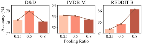
In this section, we conduct three sensitivity analyses to evaluate the impact of hyperparameters on the proposed SCHPool. First, we examine the effect of the pooling ratio on the D&D, IMDB-M, and REDDIT-B datasets, using pooling ratios k ∈ {0.25, 0.5, 0.8}. The results in Figure 2 show that datasets with lower clustering coefficients, such as REDDITB, benefit from higher pooling ratios. This is because the nodes in these graphs are sparsely distributed, leading to clusters that contain less node information. A smaller pooling ratio causes a rapid reduction in graph size, resulting in the loss of node information, thereby degrading model performance.
Next, we investigate the impact of the number of pooling layers on the D&D and IMDB-B datasets, with pooling layers L ∈ {1, 2, 3, 4} (as shown in Figure 3). The results suggest that the optimal number of pooling layers is related to the graph size. For larger graphs, such as those on the D&D dataset, more pooling layers are required to capture the structural characteristics of the graph.
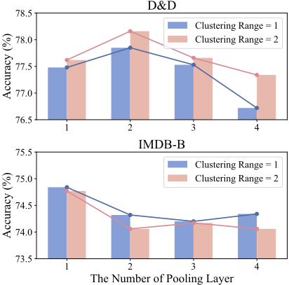
Finally, we assess the influence of the clustering range on model performance by testing ranges H ∈ {1, 2} on the D&D and IMDB-B datasets. As shown in Figure 3, graphs with higher average clustering coefficients, such as IMDB-B, benefit from a smaller clustering range due to denser node connections. A larger clustering range, in contrast, may incorporate irrelevant node information into the clusters, compromising locality and impairing model performance.
5 Conclusion
In this paper, we have proposed a novel hierarchical pooling method, SCHPool, for graph classification. Unlike existing cluster-based pooling approaches, the proposed SCHPool eliminates the need to compute complex and dense assignment matrices, significantly improving the computational efficiency. Moreover, it integrates a lightweight yet multi-view attention mechanism that adaptively aggregates both the node features within clusters and the edge connectivity strengths between clusters, resulting in more informative coarsened graphs and further enhancing model performance. Experiments demonstrate the effectiveness of the proposed method.
A Proof
Under the assumption that the components of the neighborhood conditional distribution of each node are independent and follow a Gaussian distribution, i.e,
with
The neighborhood information gain of each node can be served as an approximate empirical estimation of its neighborhood conditional entropy.
Proof.
Acknowledgments
This work is supported by the National Natural Science Foundation of China under Grants T2122020, 61602535, U21A20473, and 62172370. This work is also supported in part by the Humanity and Social Science Foundation of Ministry of Education (24YJAZH022), and the Program for Innovation Research in the Central University of Finance and Economics.
@inproceedings{ijcai2025p408,
  title     = {An End-to-End Simple Clustering Hierarchical Pooling Operation for Graph Learning Based on Top-K Node Selection},
  author    = {Zhao, Zhehan and Bai, Lu and Li, Ming and Cui, Lixin and Du, Hangyuan and Wang, Yue and Hancock, Edwin},
  booktitle = {Proceedings of the Thirty-Fourth International Joint Conference on
               Artificial Intelligence, {IJCAI-25}},
  publisher = {International Joint Conferences on Artificial Intelligence Organization},
  editor    = {James Kwok},
  pages     = {3670--3679},
  year      = {2025},
  month     = {8},
  note      = {Main Track},
  doi       = {10.24963/ijcai.2025/408},
  url       = {https://doi.org/10.24963/ijcai.2025/408},
}
TY - CPAPER TI - An End-to-End Simple Clustering Hierarchical Pooling Operation for Graph Learning Based on Top-K Node Selection AU - Zhao, Zhehan AU - Bai, Lu AU - Li, Ming AU - Cui, Lixin AU - Du, Hangyuan AU - Wang, Yue AU - Hancock, Edwin T2 - Proceedings of the Thirty-Fourth International Joint Conference on Artificial Intelligence, IJCAI-25 PB - International Joint Conferences on Artificial Intelligence Organization PY - 2025 SP - 3670 EP - 3679 DO - 10.24963/ijcai.2025/408 UR - https://doi.org/10.24963/ijcai.2025/408 ER -Copied
Machine-readable versions of this paper, for tools and AI agents:





