Online Housing Market

1 Introduction

Allocating indivisible resources to agents is a fundamental problem in computational social choice, situated at the intersection of economics [Thomson, 2011] and computer science [Klaus et al., 2016; Manlove, 2013]. The decision-maker in such problems must account for both the preferences of the agents over the resources and their strategic behavior. In this paper, we focus on a specific problem known as the housing market in the matching theory literature [Shapley and Scarf, 1974], where each agent is endowed with a single resource they are willing to exchange for another. Additionally, we assume that no monetary compensation is allowed to offset any unfavorable exchanges during the process. Despite its simplicity, this problem has numerous applications, including the exchange of dormitory rooms among students [Chen and S¨onmez, 2002], the trade of used items [Swapz, 2025], kidney exchanges where incompatible donor/recipient pairs exchange organs for transplants [Ferrari et al., 2015], and more (see, e.g., [Bir´o, 2017] for additional applications).

In this paper, we assume that preferences over resources are ordinal. The procedure for reallocating resources among agents is centralized, with the decision-maker aiming to produce an allocation that is as efficient as possible. Under ordinal preferences, Pareto optimality serves as an appropriate efficiency measure, seeking allocations where no agent can be made better off without disadvantaging another. In the standard offline setting, this requirement can be met using the serial dictatorship procedure, also known as the picking sequence [Bouveret and Lang, 2014]. In this procedure, agents are arranged in a specific order, and each agent, one by one, selects their most preferred resource from the pool of remaining resources. However, this process is not individually rational, as some agents may end up with resources less desirable than their initial endowments. This is problematic, as agents might be discouraged from participating in the trade to avoid being worse off. The well-known Gale's top trading cycle (TTC) procedure [Shapley and Scarf, 1974] addresses this issue by ensuring individual rationality while producing a Pareto-optimal allocation.

Since the procedure is centralized, the decision maker must interact with agents to gather their preferences over resources. However, during this process, agents may misreport their preferences in an attempt to manipulate the procedure and achieve a more favorable outcome. Mechanism design seeks to create procedures where truthfully revealing preferences is a dominant strategy for agents[Hurwicz and Reiter, 2006]. Both the serial dictatorship and TTC procedures possess this property. Moreover, it has been proven that the TTC procedure is the only mechanism that is simultaneously individually rational, Pareto efficient, and strategy-proof[Ma, 1994].

The standard offline setting assumes that all agents participating in the exchange are available at the same time, and that the exchange procedure is conducted during this period. However, in many contexts, this requirement is unrealistic or too demanding. In more realistic scenarios, agents are only available during restricted time periods, meaning that some may not be able to participate in the exchange simultaneously. This is the case, for example, with online exchange websites[Swapz, 2025], where agents do not arrive at the marketplace at the same time and cannot remain indefinitely before their swaps take place. This type of scenario is referred to as online[Albers, 2003], or dynamic, in the context of matching[Baccara and Yariv, 2021].

Outline. Section 2 lists related works connected to the online problem under consideration. Section 3 defines the main properties we aim to achieve. Section 4 presents online mechanisms based on the serial dictatorship procedure, while Section 5 introduces multiple online variants of the TTC procedure.

2 RelatedWorks

Multiple social choice problems have been examined through the lens of online procedures. In fair division, which aims to allocate resources fairly, several online variants have been explored[Aleksandrov and Walsh, 2020; Sankar et al., 2021; Hosseini et al., 2024]. For instance, strategy-proofness and Pareto efficiency have been studied in this context[Aleksandrov et al., 2015], along with envy-freeness. Various extensions of the serial dictatorship procedure have been proposed to achieve these properties[Aleksandrov and Walsh, 2019]. The online electric vehicle charging problem[Gerding et al., 2019], which focuses on scheduling charging for customers arriving in an online fashion, also shares similarities with our problem. However, in both cases, the online setting differs from ours, as resources do not arrive dynamically and are known to the procedure from the outset. Closer to our setting, as it addresses a one-to-one matching problem, an online version where preferences are elicited incrementally by querying agents has been considered[Hosseini et al., 2021]. A procedure that elicits preferences to achieve Pareto-optimality while minimizing the number of queries has been proposed.

Numerous works have focused on dynamic kidney exchange[ ¨Unver, 2010; Ashlagi and Roth, 2021], where donors and recipients arrive in an online fashion. Most of these studies consider compatibility (0-1 preferences) rather than ordinal preferences. Additionally, they often assume that the allocation process can be probabilistic, rely on probabilistic assumptions about arrivals and departures, and aim to reduce the expected waiting time before a transplant[Bloch and Cantala, 2017; Anderson et al., 2017; Baccara et al., 2020]. Other studies focus on maximizing the expected number of matched pairs[Awasthi and Sandholm, 2009; Dickerson et al., 2012]. The design of strategy-proof and individually rational mechanisms has also been considered for transplant centers participating in national exchange programs[Ashlagi et al., 2015; Hajaj et al., 2015].

3 Preliminary

Let N = {1, . . . , n} denote the set of agents. Each agent i owns a single good 1 ei, called her initial endowment. Let T = [t-, t+] denote the timeline during which the market is open, where t- and t+ represent the opening and closing times, respectively. For each agent i, ai and di represent her (earliest) arrival and (latest) departure times in the market, with ai, di ∈ T such that t- ≤ ai < di ≤ t+. To simplify the setting, we assume that no two arrival or departure times occur simultaneously. Let E = {e1, . . . , en} represent the set of items. Each agent i has a strict ordinal preference ≻i over the items in E, such that ej ≻i ek means agent i strictly prefers ej over ek. Furthermore, symbol ⪰i stands for ≻i or =. An instance of the online exchange problem is represented by the set of tuples {(i, ei, ai, di,≻i)}i∈N. Without loss of generality, we assume that the agent indices are ordered by increasing arrival times, i.e., such that a1 < a2 < . . . < an hold. Let I denote the entire set of possible instances.

Our goal is to allocate to each agent a single item such that each item is assigned only once. In other words, we search for an allocation M : N → E such that M(i) ̸= M(j) for each i ̸= j. The timeline constraints are such that each agent will leave the market with an item which belongs to an agent that arrived in the market earlier than her departure time. For any t ∈ T , let N<t = {i ∈ N : ai < t} denote the subset of agents arriving before t. For a given instance I, an allocation M is I-compatible if M(i) ∈ E<di holds ∀i ∈ N, where E<t = {ei : i ∈ N<t} for each t ∈ T . For any instance I, the set of I-compatible allocations is denotedM(I).

1 The resources are interchangeably referred to as goods or items

An exchange algorithm A returns an I-compatible allocation for each instance I. We assume that Ai(I) denotes the item allocated to agent i by algorithm A for instance I. In the online version of the problem, the algorithm should make a decision on the allocation for an agent when she leaves the market, without knowing the agents that arrive after her departure. In other words, the mechanism should make a decision only based on the agents that already visited the market by the departure time of the agent. For any t ∈ T , let I<t denote a truncated copy of I restricted to the agents of N<t.

Definition 1. An exchange algorithm A is online if for each instance I and for each agent i, Ai(I) = Ai(I<di ) holds.

The choice between online exchange algorithms should be guided by the properties fulfilled by the allocation that they compute. To compare these algorithms, we consider multiple standard desiderata properties. The first one is a standard definition of efficiency in multi-agent problems.

Definition 2. AllocationM ′ Pareto-dominates allocationM if for each agent i, M ′ (i) ⪰i M(i), and for at least one agent j, M ′ (j) ≻j M(j). For a given instance I, let S denote a subset of M(I). Allocation M is S-Pareto optimal (S-PO), if there is no allocationM ′ of S that Pareto-dominates it.

The standard notion of Pareto optimality corresponds to M(I)-PO, as illustrated by the following example.

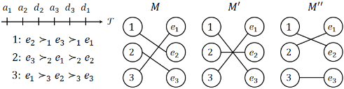
Example 1. Consider instance I described in Figure 1. The timeline, containing the arrival and departure times of the agents, as well as their preferences are in the left part of the figure. Three different allocations are provided in the right part of the figure. For example, allocation M is such that M(1) = e2, M(2) = e3, and M(3) = e1. Note that M is not I-compatible, as agent 2 receives an item from an agent who arrives later than d2. Therefore, M does not belong toM(I). Allocations M ′ andM ′′ are I-compatible andM(I)-PO.

Restricting comparisons to I-compatible allocations allows for the existence of efficient solutions, even if better ones exist but are incompatible with the online setting.

Definition 3. Exchange algorithmA is individually rational (IR), if for each instance I, Ai(I) ⪰i ei for any agent i.

Individual rationality property incentivize agents to participate in the exchange algorithm, as no agent receive an item that is less desirable than her initial endowment. Another standard property related to the manipulative power of agents, through misreporting their preferences, is called incentive compatibility. We generalize this notion to take into account manipulations related to arrival and departure times.

Definition 4. An exchange algorithm is strongly incentive compatible (SIC), if for each agent i and for each pair of instances I and I ′ such that I ′ = I \ {i, ei, ai, di,≻i} ∪ {i, ei, a′i , d′i ,≻′i } and ai ≤ a′i < d′i ≤ di, Ai(I) ⪰i Ai(I ′ ) holds. It is a-IC (respectively d-IC) if the above inequality holds only when di = d′i (respectively ai = a′i ). 2 Finally, it is weakly incentive compatible (WIC), if the above inequality holds only when both ai = a′i and di = d′i .

The notion denoted WIC corresponds to the standard incentive compatibility in the offline case. Stronger notions should incentivize agents to arrive as early as possible (a-IC), as late as possible (d-IC), or both (SIC). We assume that ai and di are agent i's earliest arrival and latest departure times, so she cannot arrive earlier than ai or depart later than di. Definition 4 states that agent i cannot benefit by arriving later than ai or departing earlier than di under an SIC mechanism.

4 Serial Dictatorship Procedure

In this section, we consider an exchange algorithm based on the serial dictatorship procedure, which is described in Algorithm 1. The standard version of the serial dictatorship procedure is based on a permutation of the agents defining the order in which each agent will choose her item among the remaining ones. We slightly generalize these permutations by considering permutation functions whose order depends on the instance. More formally, Π : I → N N denotes this permutation function, which is such that for any instance I and for any i ∈ {1, . . . , n}, Πi(I) denotes the agent choosing at position i. We assume here that this permutation function only depends on the arrival and departure times of the agents. An example of such a permutation is the ascending departure permutation δ which ranks the agents according to their departure times, 3 and more specifically by increasing departure times, i.e., such that dδ(1) < dδ(2) < . . . < dδ(n).

In Algorithm 1, every iteration of the "for" loop corresponds to the departure of an agent, specifically agent δ(i), whose departure time is the ith earliest. However, the order in which the agents choose their items is determined by the permutation function Π. Therefore, before agent δ(i) chooses her item, all agents that are ranked before her according to Π must choose their items. Once an agent has chosen an item, she is permanently matched to it, even if more desirable items arrive later. Note that the procedure besti returns the most preferred item of agent i from a given set of items.

Algorithm 1 is designed to be online, as only the part of the instance corresponding to agents who have already arrived, I<dδ(i) , is used at iteration i, during the departure of agent

2 The notion of participation in [Mattei et al., 2017] is close to aIC, except that it does not require standard incentive compatibility.

3 The input instance is omitted to simplify notations.

Algorithm 1 Online serial dictatorship procedure

Input: Permutation function Π.

1: Initialize M as an empty matching. 2: A← ∅. {Items already assigned.} 3: B ← ∅ {Agents already matched.} 4: j ← 1 {Position of the first remaining agent to choose.} 5: for i = 1 to n do 6: {Iteration occurring at dδ(i).} 7: if δ(i) ̸∈ B then 8: Let π denotes Π(I<dδ(i) ). 9: while π(j) ̸= δ(i) do 10: M(π(j)) ← bestπ(j)(E<dδ(i) \ A). 11: A ← A ∪ {M(π(j))}. 12: B ← B ∪ {π(j)} 13: j ← j + 1. 14: M(δ(i)) ← bestδ(i)(E<dδ(i) \ A). 15: A←A∪ {M(δ(i))}. 16: B ←B ∪ {δ(i)} 17: j ← j + 1. 18: returnM.

δ(i). However, the permutation must be prefix-consistent i.e., the order of agents already matched to items must not change when new agents arrive. Otherwise, an agent might be matched multiple times or ignored by the algorithm.

Definition 5. Permutation function Π is prefix-stable (PS), if for each agent i, and for any positions i′ and j ′ such that Πi′ (I) = i and j ′ ≤ i′ , Πj ′ (I) = Πj ′ (I<di ) holds.

The following proposition shows that Algorithm 1 is online and weakly incentive compatible with PS permutation.

Proposition 1. ⋆4 Algorithm 1 is both online and WIC if the input permutation function is PS.

4.1 The Ascending Departure Permutation

The following proposition shows that the ascending departure permutation is a good candidate to be used with Algorithm 1.

Proposition 2. ⋆ Ascending departure permutation δ is PS.

Note that when Algorithm 1 is used with the ascending departure permutation δ, the algorithm allows each agent to choose the best remaining item upon leaving the market.

Example 2. We run Algorithm 1 with the ascending departure permutation δ on the instance of Figure 1. At d2 (departure of agent 2), she selects item e1 that she prefers to e2. Then, at d3, agent 3 selects item e2 that she prefers to e3. Finally, agent 1 selects e3, which is the only remaining item. The resulting allocation is M ′ described in Figure 1.

The following proposition shows that the ascending departure permutation δ leads to a Pareto efficient outcome.

Proposition 3. ⋆ For any I ∈ I, Algo. 1 using the ascending departure permutation δ, returns aM(I)-PO allocation.

The following proposition shows that no other online exchange algorithm always returns a Pareto-efficient outcome.

4 Propositions marked with ⋆ indicate that proofs are omitted due to space limitations, but are included in the supplementary material

Proposition 4. Algorithm 1 using the ascending departure permutation δ is the only online exchange algorithm that returns for any instance I anM(I)-PO allocation.

Proof. By contradiction, let A denote an online exchange algorithm that behaves differently than Algorithm 1 with the ascending departure permutation δ. This means that there is an instance I and an agent j such that Aj(I) does not correspond to the assignment made by Algorithm 1 with permutation δ. In other words, agent j does not receive her most favorite item among those in E<dδ(j) minus the items already assigned to agents leaving earlier than her. Furthermore, we assume w.l.o.g. that, among the set of agents in this situation, agent j is the one who leaves the earliest. Let M denote the allocation obtained by Algorithm 1 with permutation δ applied to I. Let i denote the agent who receives M(j) instead of agent j in A(I), i.e., such that Ai(I) = M(j). By assumption, dj < di holds since, otherwise, an agent arriving earlier than agent j would not receive the same item as in M.

To show the contradiction, we construct a new instance I ′ by adding dummy agents to I. For any agent k leaving after dj, let k′ be a dummy agent such that ak′ = dj + kϵ, with ϵ > 0 small enough for all these agents to arrive earlier than any other arrival or departure, and dk′ large enough to leave after any other agent of I. The preferences of the agents in I ′ are as follows. For any agent k that was already in I and leaving after dj , her favorite item is ek′ , followed by the items of I ranked in the same order, and finally all other items of I ′ ranked arbitrarily. Dummy agent i′ 's preferences are Aj(I) ≻i′ M(j) ≻i′ . . ., where all the other items are ranked arbitrarily. Finally, the favorite item of other dummy agent k′ is Ak(I), and all other items are ranked arbitrarily.

Note first that since A is online, both Aj(I ′ ) = Aj(I ′<dj ) and Aj(I<dj ) = Aj(I) hold. Furthermore, since all dummy agents arrive later than dj, I<dj = I ′<dj , which implies with the former equalities that Aj(I ′ ) = Aj(I). Concerning the assignment of the other agents, based on their preferences and since A is M(I ′ )-PO, we can say that for each dummy agent k′ , we have Ak′(I ′ ) = Ak(I), and for each regular agent k leaving after dj, we have Ak(I ′ ) = ek′ . More precisely for i′ we have Ai′(I ′ ) = Ai(I) = M(j). Note that except for agents i′ and j, any agent receives her favorite item.

But now consider the almost same allocation, say M ′ , as the one constructed by A, except that agent j receives M(j) and agent i′ receives Aj(I). Note that by construction, M ′ should belong to M(I ′ ) since A is an online exchange algorithm, and therefore A(I<dj ) = A(I ′<dj ) belongs toM(I ′<dj ) (for agent j and the ones leaving after her), A(I ′ ) belongs toM(I ′ ) (for all other agents except agent i′ ), and ai′ < di holds (for agent i′ ). Agent j and dummy agent i′ receive in M ′ a strictly better item than the one offered by algorithmA. Therefore, M ′ Pareto dominates A(I ′ ), leading to a contradiction since A is M(I ′ )-PO.

Propositions 3 and 4 suggest focusing on Algorithm 1 with input δ when we want an online algorithm that returns an efficient outcome. Furthermore, Proposition 1 and 2 attest that this algorithm is WIC. However, it is easy to check that Algorithm 1 using input δ is neither a-IC, d-IC nor IR.

Corollary 5. There is no online exchange algorithm that both returns a M(I)-Pareto optimal allocation for any instance I ∈ I, and is either a-IC, d-IC or IR.

4.2 The Ascending Arrival Permutation

Another candidate is the ascending arrival permutation α, which ranks the agents by increasing arrival time i.e., such that aα(1) < aα(2) < . . . < aα(n). The following proposition shows that this permutation α is consistent with Algorithm 1.

Proposition 6. ⋆ Ascending arrival permutation α is PS.

Example 3. We run Algorithm 1 with the ascending arrival permutation α on the instance of Figure 1. At d2, agent 1 selects first and picks e2, which she prefers to e1. Then, agent 2 selects the last remaining item at d2, which is e1. Finally, at d3, agent 3 picks the last remaining item, which is e3. The resulting allocation is M ′′ described in Figure 1.

Furthermore, choosing the ascending arrival permutation α incentivizes agents to truthfully report their departure time.

Proposition 7. ⋆ Algorithm 1 is online and d-IC if and only if it uses the ascending arrival permutation α as input.

Note that this statement is not as strong as Proposition 4 since it does not rule out any other d-IC online exchange algorithm. The following proposition rules out the existence of a permutation that achieves a-IC with Algorithm 1.

Proposition 8. ⋆ There is no online permutation function that makes Algorithm 1 a-IC.

5 Top Trading Cycle Based Algorithms

We now explore the possibility to extend the TTC procedure to our online problem. This procedure is a natural candidate to achieve the properties mentioned in Section 3, since in the offline context it fulfills all of them, and even stronger requirements [Roth and Postlewaite, 1977; Ma, 1994]. Before providing an extension of TTC to the online setting, we provide a description of the standard TTC procedure in Algorithm 3, which will be used as a subroutine of our online algorithms. This procedure relies on the TTCgraph, which is an oriented graph where agents are vertices. As described in Algorithm 2, each vertex has an out-degree of one, and the single oriented edge starting at the vertex corresponding to an agent i is oriented to the vertex corresponding to agent j whose item ej is the most favorite according to ≻i among the ones detained by the agents in the graph. Such a graph should contain at least one cycle, and items are assigned along these cycles. Each agent contained in the cycle is assigned the item belonging to the agent that she is pointing to and leaves the market with this item. The procedure continues repeatedly with the remaining agents and their initial endowment until each agent is assigned an item.

It is well known that the TTC procedure is IR in the offline setting, and any online extension of this algorithm should keep this property. However, concerning the other properties, in the online setting not all agents are present at the beginning of the algorithm, and some of them will not arrive before the departure of other agents. Therefore, Algorithm 3 should be customized to fit the online setting. We explore a procedure

Algorithm 2 TTC-graph construction

Input: Subset of agents N ′ and their initial endowment. 1: V ←N ′ . {Set of vertices.} 2: H ← ⋃i∈N ′{ei}.{Houses owned by the agents of N ′ .} 3: E ← ∅. {Set of edges.} 4: for each i in N ′ do 5: E ←E ∪ (i, besti(H)). 6: return G = (V,E).

Algorithm 3 Top trading cycle algorithm

Input: Subset of agents N ′ and their initial endowments.

1: while N ′ ̸= ∅ do 2: Construct the TTC-graph G(N ′ ) using Algorithm 2. 3: for each cycle C = (c1, c2, . . . , ck) in G(N ′ ) do 4: for i = 1 to k - 1 do 5: M ′ (ci) ← eci+1 . 6: M ′ (ck) ← ec1 . 7: N ′ ←N ′ \ C. 8: returnM ′ .

described in Algorithm 4, which applies TTC to subsets of agents already present in the market, according to an input partition function. Partition function P applied to I will partition the agents of I into multiple subsets. More formally, a partition function P : I → 22N maps any instance I ∈ I to a partition P(I) of the agents in I. This means that P(I) is a collection of subsets of agents such that the union of these subsets is N, and no two subsets share an agent. We assume once again that the result of this function is independent of the preferences of the agents and their initial endowments. To construct the allocation, Algorithm 3 is applied independently to the subsets of agents returned by this partition function. To simplify notations, we assume that Pi(I) denotes the subset of P(I) that contains agent i.

The TTC procedure described in Algorithm 4 requires that an agent is not selected multiple times for application of Algorithm 3. This translates into the following property.

Definition 6. A partition function P is online compatible (OC) if for any instance I and agent i, Pi(I) = Pi(I<di ).

It is easy to check that if partition function P is OC, then for any agent i, Pi(I) contains only agents that are in the market at time di, i.e., for any j ∈ Pi(I), aj < di < dj must hold. Furthermore, no agent participates multiple times to the TTC procedure when the partition function used by Algorithm 4 is OC. The following proposition outlines the properties of OC partition functions with respect to Algorithm 4.

Proposition 9. ⋆ Algorithm 4 using a OC partition function as input is both online and WIC.

5.1 The Departing Agent Excluded Partition

We explore now if a stronger notion of incentive compatibility can be achieved with particular partition functions. Let us introduce the departing agent excluded partition γ, whose construction is described in Algorithm 5. Intuitively, every time that an unpartitioned agent leaves the market, two new

Algorithm 4 Online top trading cycle procedure

Input: Partition function P. 1: B ← ∅ {Agents already matched.} 2: for i = 1 to n do 3: {Iteration occurring at dδ(i).} 4: if δ(i) ̸∈ B then 5: Applies Algorithm 3 to Pi(I<dδ(i) ) to obtainM ′ . 6: for all j ∈ Pi(I<dδ(i) ) do 7: M(j) ←M ′ (j). 8: B ←B ∪Pi(I<dδ(i) ) 9: returnM.

Algorithm 5 Departing agent excluded partition γ

Input: Instance I = {(i, ei, ai, di, ≻i)}i∈N .

1: B ← ∅. {Set of agents belonging to the partition.} 2: γ ← ∅ {The partition to construct.} 3: for i = 1 to n do 4: {Iteration occurring at dδ(i).} 5: if δ(i) ̸∈ B then 6: γ ← γ ∪ {{δ(i)}} ∪ {N<dδ(i) \ (B ∪ {δ(i)})} 7: B ←B ∪N<dδ(i)

• 8: return γ.

subsets are added to the partition. The first is a singleton containing the agent leaving the market, and the second is the remaining unpartitioned agents that are present in the market.

Proposition 10. ⋆ The departing agent excluded partition γ is OC.

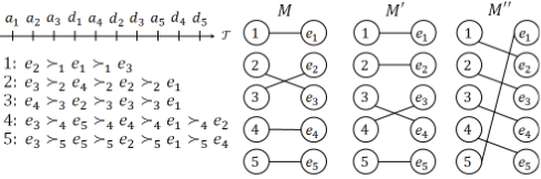
Example 4. Consider the instance I and the three allocations depicted in Figure 2. It is easy to verify that Algorithm 1 using either the ascending departure permutation δ or the ascending arrival permutation α returns allocation M ′′ , which is not IR since agent 5 receives item e1.

Let us first run Algorithm 5 to compute the departing agent excluded partition γ(I). At d1, N<d1 = {1, 2, 3}. Therefore, {1} and {2, 3} are added to the partition. At d2 and d3, nothing occurs since agents 2 and 3 are already in the partition. At d4, N<d4 = N, but agents 1, 2, and 3 are already in the partition. Therefore, {4} and {5} are added to the partition, and Algorithm 5 returns γ(I) = {{1}, {2, 3}, {4}, {5}}.

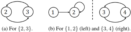
Let us now run Algorithm 4 with γ(I) as input to compute the allocation for this instance. The TTC procedure is applied only once to a subset of more than one agent, which is {2, 3}. As depicted in Figure 3a, the TTC-graph for the subset of agents {2, 3} contains a single cycle covering all agents, and they swap their goods. The resulting allocation is M.

The idea under this partition function γ is to punish agents, who force the assignment to take place because they leave earlier, by leaving them alone in the partition. The consequence for Algorithm 4 is that they keep their initial endowment without exchange. The following proposition shows more formally that no agent has an incentive to misreport her departure time when Algorithm 4 uses partition function γ.

Proposition 11. Algorithm 4 using the departing agent excluded partition γ is d-IC.

Proof. We know by Propositions 9 and 10 that Algorithm 4 with partition γ is WIC. It remains to show that no agent has an incentive to misreport her departure time. Let S denote the subset of agents for which the "if" clause of Algorithm 5 is true, i.e., agents that are not partitioned until their departure.

Consider first the case of an agent i ∈ S. Note first that agent i belongs to a singleton in the departing agent excluded partition γ. Let us show that even if agent i declares an earlier departure time d′i such that ai < d′i < di, then there is no other agent j of S such that d′i < dj < di. Indeed, since dj < di, we know that agent j is considered before agent i during the "for" loop of Algorithm 5. In the last instruction of this loop when agent j is considered, N<dj is added to the set of partitioned agents B. Since agent i is not in B at iteration di of the loop, it means that she is not in N<dj , or in other words ai > dj . This implies with ai < d′i that dj < d′i .

We now know that any agent of S leaving earlier than agent i will still leave earlier than i even after i declares a new departure time d′i . This implies that agent i will still pass the "if" test in the loop of Algorithm 5 even if she changes her departure time because no agent of S leaving earlier will include i in a partition. Therefore, agent i will be alone in the departing agent excluded partition γ after misreporting her departure time and will keep her item during Algorithm 4. So, she has no incentive to misreport her departure time.

Consider now the case of an agent i not in S. Note first that i ̸∈ S means that there is an agent j ∈ S such that dj < di and i ∈ N<dj . We assume that j is the agent of S with the lowest rank in the ascending departure permutation δ for which these inequalities are true. In other words, the subset of agents containing agent i is selected by Algorithm 5 during the iteration of the "for" loop corresponding to dj . By applying the same reasoning as above, it is easy to check that there is no agent k of S such that dk < dj and d′i < dk. Therefore, the only misreport d′i of agent i that could change the outcome of Algorithm 5 is such that dj > d′i . In that case, agent i will belong to the set of agents for which the "if" condition of Algorithm 5 is true, and therefore agent i will be alone in the departing agent excluded partition γ, and will receive her item in Algorithm 4. Since Algorithm 4 is IR, agent i has no

Algorithm 6 Scheduled departure partition θ.

• Input: Instance I, and schedule ξ = {ξ0, ξ1, . . . ξk}. 1: A← {0}. {Set of intervals of ξ already considered.} 2: B ← ∅. {Set of agents belonging to the partition.} 3: for i = 1 to n do 4: {Iteration occurring at dδ(i).} 5: Let ξj denote the interval of ξ containing dδ(i). 6: if j ̸∈ A then 7: Let S be the subset of agents of I<dδ(i) whose departure times belong to ξj . 8: θ ← θ ∪ {S}. 9: A←A∪ {j}. 10: B ←B ∪S. 11: else if δ(i) ̸∈ B then 12: θ ← θ ∪ {{δ(i)}}. 13: B ←B ∪ {δ(i)}. 14: return θ.

incentive to misreport her departure time.

Unfortunately, it is easy to check that Algorithm 4 using the departing agent excluded partition γ is not a-IC.

5.2 Partition Functions Based on Schedules

Let us now examine if a-IC can be achieved by Algorithm 4 using another partition function. To do so, we introduce a subset of non-overlapping time intervals ξ = {ξ0, ξ1, . . . , ξk}, that we call schedule. More formally, we assume that for any j ∈ {0, 1, . . . , k}, ξj ⊆ T , and for any j ′ ̸= j, ξj ∩ ξj ′ = ∅. We assume that each interval is contiguous, potentially with the exception of ξ0, which covers all time intervals not contained in the other intervals. This schedule will be used to initialize the partition by grouping agents whose departure times belong to the same time interval of ξ.

The construction of the scheduled departure partition θ is described in Algorithm 6, and depends on both the arrival and departure times of the agents, and the input schedule ξ. Intuitively, all agents whose departure times belong to the same time interval and whose arrival times are no later than the earliest departure time of one of these agents are grouped together, whereas the other agents are left alone in the partition. Interval ξ0 plays a special role since all the agents whose departure times belong to this interval are left alone in the partition. Note that this first interval may be left empty. To simplify notation, we denote by θ the scheduled departure partition resulting from Algorithm 6, without specifying the schedule used. The following proposition shows this the partition function is online compatible.

Proposition 12. ⋆ Scheduled departure partition θ is OC.

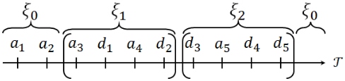
Example 5. Consider once again instance I described in Figure 2, and schedule ξ represented in Figure 4. Note that ξ1 contains the departure time of agents 1 and 2, and ξ2 contains the departure time of agents 3, 4, and 5. Let us run Algorithm 6 to compute the scheduled departure partition θ(I). At d1, both agents 1 and 2 are in N<d1 . Therefore, {1, 2} is added to the partition. At d2, nothing happens since agent 2 already belongs to the partition. At d3, both agents 3 and 4 are in N<d3 . Therefore, {3, 4} is added to the partition. At d4, nothing happens since agent 4 is already part of the partition. At d5, the interval ξ2 that contains d5 has already been considered. Therefore, agent 5 remains alone, and {5} is added to the partition. Finally, the algorithm halts and returns the scheduled departure partition θ(I) = {{1, 2}, {3, 4}, {5}}.

Let us now run Algorithm 4 using θ(I) as input to compute the allocation. The TTC procedure is applied independently to {1, 2} and {3, 4}. The TTC-graphs during the first iteration of the TTC procedure are represented in Figure 3b. The TTC-graph for the subset of agents {1, 2} (left part of Figure 3b) contains a single cycle, which is the self-loop involving agent 2. Therefore, agent 2 keeps her good, and agent 1, who remains alone during the second iteration, also keeps her good. The TTC-graph for {3, 4} (right part of Figure 3b) contains a single cycle that includes both agents, who swap their goods. The resulting matching is M ′ of Figure 2.

Note that if agents i and j have their departure times belonging to the same time interval and one of them, say i, leaves before the arrival of the other, then agent j is left alone in the scheduled departure partition θ. That was the case for agent 5 in Example 5. The underlying idea is that the set containing agent i in the partition θ must be decided before her departure, and agent j, who arrives later, cannot be included in the same set. Additionally, agent j cannot be partitioned with other agents to avoid incentivizing her to strategically delay her arrival time. The following proposition shows that no agent has an incentive to misreport her arrival time with the partition function returned by Algorithm 6.

Proposition 13. ⋆ Algorithm4 using the scheduled departure partition θ is a-IC.

Unfortunately, Algorithm 4 using the scheduled departure partition θ is not d-IC, with the exception of the schedule containing only ξ0. In that case, ξ0 = T holds and the resulting partition is the one where each agent is alone. Algorithm 4 will therefore assign to each agent her own item. This algorithm is obviously SIC since its outcome does not change with the preferences and the arrival and departure time of the agents. However, this algorithm is not really interesting since no exchanges among agents are performed, and the allocation is not improved. By combining the properties of Algorithms 5 and 6, we can create a less trivial partition function that renders Algorithm 4 SIC. To do so, we can use Algorithm 6 as a baseline, and modify line 8 by the assignment θ ← θ∪{{δ(i)}}∪{S\{δ(i)}}, which is consistent with line 5 of Algorithm 5. Furthermore, we restrict the input schedule to {ξ0, ξ1} such that ξ0 = ∅ and ξ1 = T. The resulting partition function is called earliest departure partition ζ. In other words, this partition ζ groups together all the agents of I<δ(1), with the exception of agent 1, and all the other agents stay alone. This partition ζ is easily shown to be OC due to its similarity in construction to Algorithms 5 and 6.

Example 6. Consider one last time instance I described in Figure 2. Let us compute the earliest departure partition ζ(I) by running the modified version of Algorithm 6 described in the previous paragraph. At d1, during the earliest departure time of an agent, N<d1 contains agents 1, 2, and 3. Therefore, {1} and {2, 3} are added to the partition. All the other agents will remain alone in the partition. Thus, the algorithm halts and returns the earliest departure partition ζ(I) = {{1}, {2, 3}, {4}, {5}}, which is identical to the departing agent excluded partition γ(I). Therefore, the matching returned by Algorithm 4 is M depicted in Figure 2.

Proposition 14. ⋆ Algorithm 4 using the earliest departure partition ζ is SIC.

The main drawback of the earliest departure partition ζ is that only one coalition contains more than one agent, and the exchanges performed during the TTC procedure may involve few agents. Their number depends on the agents present in the market when the first agent leaves and ranges from 1 (if a2 > d1) to n - 1 (if an < dδ(1)).

6 Conclusion and FutureWorks

We extended the serial dictatorship and TTC procedures to an online setting, aiming to develop mechanisms that are Paretoefficient, individually rational, and incentivize agents to truthfully reveal their preferences, as well as their actual arrival and departure times. Several variants of these mechanisms were proposed and are summarized in Table 1 along with their respective properties. The paper also presents additional results not summarized in Table 1. For example, we proved that Algorithm 1 using the ascending departure permutation δ is the only mechanism always returning a M(I )-P O allocation.

An intriguing extension of this work would be to explore dynamic versions of these mechanisms, where the allocation of an agent remaining in the market could evolve even after an item has been assigned to her. Another promising direction is the design of a strongly incentive-compatible mechanism that enables more exchanges than Algorithm 4 with the earliest departure partition ζ. Lastly, we could investigate relaxed forms of efficiency and strategy-proofness, potentially incorporating probabilistic assumptions about arrival patterns. Such probabilistic assumptions are closely related to the online stochastic matching problem [Feldman et al., 2009; Huang and Shu, 2021]. A similar approach has also been explored for the fair assignment of public goods [Banerjee et al., 2022; Banerjee et al., 2023].