Logarithmic Approximations for Fair k-Set Selection

1 Introduction

The problem of fair k-set selection is to select k sets from a given set system such that the (weighted) occurrence times that each element appears in these k selected sets are balanced, i.e., the maximum (weighted) occurrence times among all elements are minimized. Observe that a set system can be formulated into a bipartite graph G := (L ∪ R, E), i.e., each element and set corresponds to a vertex in L and R respectively; there is an edge between an element vertex and a set vertex if the element is included in the set. Thus, the fair k-set selection problem is equivalent to finding k vertices from R such that the maximum (weighted) number of selected neighbors of vertices in L are minimized.

The above problem aims to balance the frequency of element occurrence within a selected subset of sets. Thus, it falls under the umbrella of the subset selection problem, which arises in a wide range of applications in various fields, such as artificial intelligent [De and Chakrabarti, 2022; Mehrotra and Vishnoi, 2023; Tschiatschek et al., 2017], machine learning [Boehmer et al., 2023; Lang et al., 2022; Mirzasoleiman et al., 2020; Tukan et al., 2023], data mining [Bao et al., 2022; Yi et al., 2023], operations research [Hazimeh and Mazumder, 2020; Mazumder et al., 2023], to name just a few. In the following, we present three concrete applications of the problem in the recommended system, feature selection, and facility location. As a typical application of subset selection algorithms, our problem also captures applications in feature selection on unbalanced datasets, which is described in the full version of the paper [Li et al., 2025].

Fair Ad Recommendation. The first application of the above problem is about ad recommendation. Fairness plays a vital role in recommendation systems and an unfair system may harm the benefits of multiple stakeholders [Abdollahpouri and Burke, 2019; Beutel et al., 2019; Li et al., 2023]; see [Wang et al., 2023] for an excellent survey. The fair k-set selection problem can model a fair ad recommendation scenario as follows: a recommendation system has n users, and the company needs to select k types of ads from m types to push to these users. A user may dislike some ad types, and this can be learned from her block history. If the user receives too many ads that she does not like to see, this will cause her to resent the recommendation system. We use disagreement to denote the case where a user sees an ad that she dislikes. The goal is to fairly pick k ads fromm ads, i.e., minimize the maximum disagreement among all users.

Fair Facility Location. The last impetus for studying the above problem is an application in facility location. Fairness in facility location has been extensively studied in the field of both game theory and computational social choices [Aziz et al., 2022; Wang et al., 2021; Zhou et al., 2022]. Consider the following scenario where the government aims to select k positions fromm positions to build facilities (e.g., garbage recycle stations). There are n agents, and all agents do not want many garbage recycling stations built near them. Each agent has multiple adjacent positions, which can be viewed as a subset of the given m positions. We also use the disagreement to denote that case where some recycling station is built near an agent. The goal is to find a fair way to build k facilities, i.e., minimize the maximum disagreement.

Our problem is related to the anonymous refugee housing problem, which was recently proposed by [Knop and Schierreich, 2023; Schierreich, 2023]. In this problem, the input is an undirected graph, and each vertex corresponds to a house that is either an empty house or occupied by an inhabitant. There are k anonymous refugees, each of which is required to be assigned an empty house. Each inhabitant has an upper bound, and an assignment is called inhabitant respected if the number of refugees in the neighborhood of every inhabitant is at most its upper bound. The goal is to determine whether an inhabitant-respected assignment exists. By considering (i) each inhabitant as an element; (ii) each empty house as a set of inhabitants that are adjacent to this empty house, the minimax fairness version of the anonymous refugee housing problem is equivalent to our problem. So, the fair anonymous refugee housing problem can be viewed as another application in Fair Facility Location. The previous works only focus on the computation complexity while we aim to design approximate algorithms, and this leads to a completely different technique.

For convenience of description, we mainly use the bipartite-graph-based formulation of our problem. By following the convention of the computational social choice community, we consider each vertex in L as an agent and the integer k as the demand, where k is the number of vertices that we need to select. For each vertex in L, we use disagreement to denote the number of selected neighbors of this vertex. The formal definition of the problem is shown in Section 2.

1.1 Our Contributions

We consider the Fair k-Set Selection problem (FKSS) in which we mainly use the bipartite graph G := (L ∪ R,E) to describe the input. We distinguish several cases according to the type of the input bipartite graph. For each case, we give either an exact or approximation algorithm running in polynomial time. In the following, we summarize the main results of this work.

Main Result 1. The problem FKSS is NP-hard even on bipartite graphs with ∆ = 3. For bipartite graphs with ∆ = 2, the problem FKSS is in P. The problem is also in P if the input set system forms a laminar family. Moreover, the maximin criteria do not admit any polynomial time α-approximate algorithm unless P = NP, where α is an arbitrary function of the input.

Our first result focuses on the computation complexity of the problem. This part is completely omitted in this version due to the space limit and can be found in [Li et al., 2025]. We first show that the problem is NP-hard even in the case ∆ = 3. The hardness result is built on the maximum independent set on planar graphs, which is shown to be NP-hard in [Garey and Johnson, 1977]. We then show that the complement case (∆ = 2) is polynomially solvable by giving a simple and efficient combinatorial algorithm. For the laminar set family, we give a dynamic programming algorithm that computes the optimal solution in polynomial time. One may expect that maximin criteria are also candidates to investigate the fairness of the k-set selection problem. Namely, find k sets such that the minimum number of selected neighbors of vertices in L is maximized, where we call these neighbors agreement. This is not the case because it is NP-hard to determine whether the optimal solution has a zero agreement; this case is equal to determining whether there exist k sets that cover all elements.

Main Result 2 (Theorem 1, 2). Given any instance of FKSS on general bipartite graphs, there is a randomized algorithm that achieves O( logn log log n )-approximation with high probability running in poly(n) times, where n is the number of vertices in the graph. Moreover, our analysis is optimal up to a constant factor.

Our second result focuses on the general bipartite graph (Section 3). To have a better understanding of our algorithmic ideas, we focus on the unweighted case in Section 3, and then we extend our algorithms to the weighted case in [Li et al., 2025]. We give two algorithms and both algorithms are LP-based rounding algorithms. The first algorithm is a simple independent rounding algorithm that is O( logn log log n )- approximate and it only can satisfy the demand requirement with high probability. The second algorithm is a dependent rounding algorithm which can surely satisfy the demand requirement while achieving the same ratio. The random variables used in the second algorithm are negatively correlated, which enables us to use the strong concentration bounds (e.g., Chernoff bound). The algorithm is a special case of the classical pipage rounding technique [Chekuri et al., 2010], which is used to handle the more general matroid constraints. We also demonstrate that our analysis is tight up to some constant factor by showing that the LP has a Ω( logn log logn ) integrality gap. This part is omitted in this version.

Main Result 3 (Theorem 3). Given any instance of FKSS on bipartite graphs with a maximum degree ∆, there is a randomized algorithm that achieves O(log ∆)-approximation with running time poly(n) in expectation. Moreover, our analysis is nearly tight.

By observing that the maximum degree of many practiced in real-life scenarios is often small compared to the number of vertices in the whole graph, our third result focuses on graphs with a maximum degree ∆ (Section 4). To have a better understanding of our algorithm, we first focus on the unweighted case in Section 4 and then extend our algorithms to the weighted case in [Li et al., 2025]. We prove that there is a randomized algorithm achieving O(log∆)- approximation ratio, which significantly improves the ∆ approximation achieved by a trivial algorithm. Our algorithm is based on the same linear programming formulation as the general graph. To get rid of the dependency on the number of vertices, we employ the powerful Lov´asz Local Lemma. Our analysis is also almost tight since the same integrality gap instance also implies a Ω( log∆ log log∆ ) gap of the natural linear programming.

1.2 Other RelatedWorks

Subset selection has numerous variants in literature. To the best of our knowledge, FKSS is a novel problem and has never been addressed before. One of the most representative subset selection problems is to select a subset of elements such that a monotone submodular function is optimized. If the selected subset is required to satisfy a cardinality constraint, the submodular maximization admits a (1- 1e )- approximate algorithm [Nemhauser et al., 1978]. This result can be further extended to a more general matroid constraint, and the approximation ratio remains the same [C˘alinescu et al., 2011; Filmus andWard, 2014]. In contrast, the submodular minimization subject to some constraint has a strong lower bound [Svitkina and Fleischer, 2011]. When the selected subset is required to satisfy a knapsack constraint, the submodular maximization also admits a (1 - 1e )-approximate algorithm [Sviridenko, 2004].

1.3 Roadmap

In Section 2, we give a formal definition of our problem. In the full version [Li et al., 2025], we show that our problem is NP-hard even if ∆ = 3, and we give a simple polynomialtime algorithm that solves the ∆ = 2 case. We also show that the problem is in P when the input set system forms a laminar family. In Section 3, we consider the problem on general bipartite graphs and give O( logn log log n )-approximate algorithms. In Section 4, we show that the problem admits a O(log∆)- approximate algorithm on graphs with a maximum degree ∆. In the full version, we extend our logarithmic-approximation algorithms in Section 3 and Section 4 to the weighted case. For a better understanding of our algorithm, we will focus on the unweighted version of our problem when presenting our logarithmic approximation algorithms.

2 Preliminaries

We consider the Fair k-Set Selection problem (FKSS) and mainly use the bipartite-graph-based formulation. An instance of FKSS consists of a bipartite graph G := (L∪R, E) with |L| = n and |R| = m and a positive integer k with k ≤ |R|, where k is called the demand. Each vertex v in R has a non-negative weight wv. When all wv are equal, we refer it to unweighted case. A feasible solution S ⊆ R is a subset of vertices in R with |S| ≥ k. In the corresponding set system, each vertex in L represents an element and each vertex in R corresponds to a set. So, we aim to choose at least k sets if we use the set system description. For each vertex i in G, let NG(i) be the set of neighbors of i in G. The disagreement of a vertex i ∈ L is the total weight of its neighbors that are also in S, i.e., disi(S) := ∑v∈NG(i)∩S wv. The goal is to select a subset of vertices S ⊆ R with |S| ≥ k such that maxi∈L disi(S) is minimized. In the remainder of this paper, we will use ∆ to denote the maximum degree of the input bipartite graph G = (L ∪ R, E), i.e., ∆ := maxi∈L∪R|NG(i)|.

3 General Graphs

In this section, we give two logarithmic approximate algorithms. To have a better understanding of our algorithmic idea, we shall focus on the case where all vertices in R have the same weight. We will extend our algorithms to the general FKSS instance in [Li et al., 2025]. Both algorithms are LP-based randomized rounding algorithms. The first algorithm is a simple independent rounding algorithm that (i) achieves O( logn log log n )-approximation with high probability; (ii) satisfies the demand requirement with high probability; see Section 3.2 for details. The second algorithm is a dependent rounding algorithm which strictly improves the first algorithm, i.e., it (i) achieves O( logn log log n )-approximation with high probability; (ii) satisfies the demand requirement with probability 1. Due to the space limits, this part is omitted in this version. The dependent rounding algorithm is a special pipage rounding algorithm proposed by [Chekuri et al., 2010], which preserves the negative correlation property. Compared to dependent rounding, independent rounding is simple and easy to analyze. The analysis of special pipage rounding requires proof of negative correlation property. In the full version [Li et al., 2025], we also show that our analysis is optimal up to the constant factor by giving a hard instance, i.e., the linear programming formulation that we used has an integrality gap of Ω( logn log log n ).

3.1 LP Formulation

The intuitive linear programming formulation is to add the objective "min T" to (Feas-LP); if so, the integrality gap shall be Ω(n). The detailed discussion is deferred to the full version. In the following, we shall use the feasibility-checking LP (Feas-LP), which is a standard technique to cut the integrality gap.

We shall guess the value of the optimal solution whose range is from 1 to k. Hence, (Feas-LP) eliminates the bad instance of the intuitive LP because the guessed value T ≥ 1. Let T ∗ be the minimum integer in [1, k] to make (Feas-LP) admit a feasible solution; T ∗ can be obtained by solving O(log k) times (Feas-LP). Observe that T ∗ is a lower bound of the optimal solution, i.e., any optimal integral solution has a maximum disagreement of at least T ∗ . Let x∗ := (x∗v )v∈R be the solution to (Feas-LP) that achieves T ∗ .

3.2 Independent Rounding

In this section, we show that there is a simple independent rounding algorithm that (i) achieves O(log n)-approximation with high probability; (ii) satisfies the demand requirement with high probability. Formally, we aim to prove the following theorem (Theorem 1).

Theorem 1. There is a randomized independent rounding algorithm that (i) achieves O( logn log log n )-approximation with probability at least 1 - 1n ; (ii) satisfies the demand requirement with probability at least 1 -O(1/ logn log log n ), where n is the number of vertices in the input bipartite graph.

Algorithmic Intuition. The algorithmic idea of Algorithm 1 is simple. We first solve (Feas-LP) to obtain a fractional solution (x∗v )v∈R, and then, we interpret x∗v as the probability that we choose v. To ensure that we can sample a sufficient number of vertices from R, we raise the probability that we choose v to O( lnn ln ln n ) · x∗v . Then, by using the Chebyshev bound, we can show that the sampled solution satisfies the demand requirement with high probability. Meanwhile, the disagreement of each vertex in L will also be raised to O( lnn ln lnn ) · T ∗ , where T ∗ is a lower bound of the optimal solution. By using the right tail Chernoff bound and union bound, we can show that the disagreement of all vertices in L is at most O( lnn ln ln n ) · OPT with high probability.

Algorithm 1 Independent Rounding Algorithm.

Input: The fractional solution x∗ .

Output: A set of vertices S ⊆ R with |S| ≥ k with high probability. 1: A← {v ∈ R : x∗v ≥ ln lnn 10 ln n }; 2: B ← {v ∈ R : x∗v < ln lnn 10 ln n }; B′ ← ∅. 3: if ∑v∈B x∗v ≤ 1 then 4: B′ ← {u}; u is an arbitrary vertex in B. 5: end if 6: if ∑v∈B x∗v > 1 then 7: for each v ∈ B do 8: pv ← 10 ln n ln lnn · x∗v . ▷ Note that pv ≤ 1. 9: Independently add v to B′ with probability pv. 10: end for 11: end if 12: return S ←A∪B′ .

In the following, we show that the returned solution of Algorithm 1 satisfies the demand requirement (Lemma 1) and ratio requirement (Lemma 2) with high probability. In the following proof, we will use the same notations stated in Algorithm 1.

Lemma 1. Algorithm 1 returns a vertex set that satisfies the demand requirement with probability at least 1-O(1/ lnn ln ln n ), where n is the number of vertices.

Lemma 2. Pr[|NG(u) ∩ B′ | ≥ 10 lnn ln lnn · T ∗ ] ≤ 1 n2 for all vertices v ∈ L.

Theorem 1 can be proven by Lemma 1 and Lemma 2 with the union bound applied. The formal proofs of these lemmas are omitted in this version.

As we have seen above, independent rounding allows us to use the strong concentration bounds but it may not be able to guarantee that the total number of selected vertices satisfies the demand. Fortunately, several dependent rounding techniques can ensure the negative correlation property with which the strong concentration bounds are still applicable. One of the most elegant methods is called pipage rounding proposed by [Chekuri et al., 2010]. The initial pipage rounding technique in [Chekuri et al., 2010] is used to handle the matroid structure. In our problem, the constraint can be viewed as a simple uniform matroid. Thus, we can obtain the following theorem via the pipage rounding algorithm. More details can be found in [Li et al., 2025].

Theorem 2. Given any instance of FKSS on general bipartite graphs, there is a randomized algorithm with running time poly(n) that (i) satisfies the demand requirement with probability 1; (ii) returns a O( logn log log n )-approximate solution with probability at least 1 - 1n , where n is the number of vertices in the input bipartite graph.

4 Graphs with Bounded Degree

In this section, we consider FKSS on the graphs with a maximum degree ∆ and mainly show that there is a O(log∆)- approximate algorithm (Theorem 3). Similar to Section 3, to have a better understanding of our algorithmic ideas, we shall focus on the unweighted case. We will extend our algorithms to the general FKSS instances in [Li et al., 2025]. We remark that our analysis is almost tight since (Feas-LP) also has an integrality gap Ω( log∆ log log ∆ ).

Theorem 3. Given any instance of FKSS on graphs with a maximum degree ∆, there is a randomized algorithm with running time poly(n) in the expectation that returns a O(log∆)-approximate solution, where n is the number of vertices in the input bipartite graph.

In practice, the maximum degree of many graphs is often small compared to the number of vertices in the whole graph. The graph with a maximum degree ∆ admits a trivial ∆-approximate algorithm. Namely, arbitrarily picking kvertices from R is a ∆-approximate algorithm by observing the following two simple facts: (i) the optimal solution to the given instance is at least 1; (ii) the maximum disagreement of any algorithm is at most ∆ since the maximum degree is ∆. However, if we use the algorithm for general graphs, we can only obtain a O( logn log logn )-approximate solution; this is not even a constant factor when ∆ is a constant. In this section, we give a O(log∆)-approximate algorithm, which significantly improves the ratio of the trivial ∆-approximate algorithm.

Main Obstacles and Our Ideas. Our algorithm is still based on (Feas-LP). To get rid of the dependency of n on the approximation ratio, there are three main obstacles that we need to overcome. The first obstacle comes from the union bound we used in the proof of Theorem 2. For each vertex u ∈ L, we define the following event as a "bad event": the disagreement of vertex u is larger than α · OPT for some parameter α. To ensure that these bad events do not occur at the same time, we need to use the union bound over all vertices in L; thus, we have to lose the factor n on the approximation ratio. However, if we do the analysis more carefully, we may realize that these bad events are not so independent. For example, assuming that two vertices u, v in L have the same set of neighbors in R. If the bad event of u does not occur, this shall imply that the bad event of v does not occur either. Based on this observation, we may not need to do union bound over all vertices, so bypassing the dependency of n. To this end, we shall use the powerful Lov´asz Local Lemma; see Section 4.1 for the definition of the lemma.

The next two obstacles come from the use of the Lov´asz Local Lemma. The second obstacle is that the Lov´asz Local Lemma requires us to do independent rounding, but the independent rounding cannot ensure the feasibility of the solution, i.e., it cannot ensure the algorithm selects at least k vertices. Our idea to overcome this obstacle is that, aside from defining a bad event for the approximation ratio, we also define a bad event for the feasibility. In this way, as long as the Lov´asz Local Lemma ensures all bad events do not occur, we obtain a solution that achieves the desired approximation ratio and satisfies the demand requirement simultaneously. The third obstacle comes from the implementation of the above feasibility idea. Namely, we need to find an appropriate definition for the feasibility bad events so that (i) all feasibility bad events do not occur, ensuring a solution that satisfies the demand requirement; (ii) the defined bad events should not dependent on many other bad events to get rid of the dependency on n. Our idea for this obstacle is a grouping technique; see Definition 1 for details.

4.1 Lov´asz Local Lemma

There are several versions of Lov´asz Local Lemma. In our work, we shall use the variable version proposed by [Moser and Tardos, 2010]. In this version, there is an underlying family of mutually independent random variables on a common probability space, denoted by X := {X1, . . . ,Xm }. Let A := {A1, . . . ,An } be a set of bad events. Each bad event Ai is determined by a subset Ai ⊆ X of variables in X. The dependency graph G := (V, E) for A is an undirected graph such that (i) each vertex v ∈ V corresponds a bad event Av in A; (ii) there is an edge between u ∈ V and v ∈ V if and only if Au ∩Av ̸= ∅. For each bad event Ai, let N(Ai) ⊆ A be a set of bad events that are adjacent to Ai in the dependency graph G.

Lemma 3 (Lov´asz Local Lemma [Moser and Tardos, 2010]). If there exists a real number xi ∈ (0, 1) for each bad event Ai ∈ A such that Pr[Ai] ≤ xi ∏Aj∈N(Ai) (1 - xj) for all Ai ∈ A, then (i) there exists an assignment of the random variables in X such that Pr[∧i∈[n]¬Ai] > 0; (ii) there exists an algorithm that finds such an assignment for X in expected time ∑i∈[n] xi 1-xi .

The algorithm proposed by [Moser and Tardos, 2010] is a simple local search algorithm; let LocalSearch(·, ·) represent this algorithm. It takes two parameters as the input: the independent random variables X and the bad events A, and it outputs an assignment X of X that makes all bad events in A not occur. Let d be the maximum degree of the dependency graph G. By setting xi = 1 d+1 for each i ∈ [n], the Lov´asz Local Lemma can be simplified, which produces the Symmetric Lov´asz Local Lemma. The symmetric Lov´asz Local Lemma was first proposed by [Erdos and Lov´asz, 1975].

Lemma 4 (Symmetric Lov´asz Local Lemma [Erdos and Lov´asz, 1975]). Let A = {A1, . . . ,Am } be a set of bad events with Pr[Ai] ≤ p for all i ∈ [n]. If e · p · (d + 1) ≤ 1, then Pr[∧i∈[n]¬Ai] > 0.

Lemma 3 implies Lemma 4. More discussions about Lemma 3 and Lemma 4 can be found in the full version.

4.2 Rounding Algorithm

Algorithm 2 is an independent rounding algorithm that is built based on the local search algorithm for Lov´asz Local Lemma (LocalSearch(·, ·)). As is typical, we interpret each variable in the optimal fractional solution x∗ = (x∗v )v∈R as the probability. For each v ∈ R, we raise the probability of the event that selects v to O(ln∆) · x∗v (see line 2 of Algorithm 2). Algorithm 2 consists of three phases: (Phase 1) Fixed Choice Phase (lines 4-7 of Algorithm 2); (Phase 2) Local Search Phase (lines 8-18 of Algorithm 2); (Phase 3) One Vertex Phase (lines 19-22 of Algorithm 2). In the first phase, we select all vertices whose probability is 1. If the number of selected vertices already satisfies the demand requirement (line 5 of Algorithm 2), then we stop; otherwise, we enter the second phase to select more vertices. Due to some technical reason, Algorithm 2 may not be able to select sufficient vertices at the end of the second phase. Fortunately, such a demand gap is at most 1. Thus, Algorithm 2 enters the third phase and arbitrarily selects one vertex.

The choice of the scaling factor O(ln∆) is crucial to the Lov´asz Local Lemma, i.e., it ensures that the probability of the bad events (which will be defined in Definition 1) satisfies the conditions stated in Lemma 4. So, we can employ LocalSearch(·, ·) to find the right selection of vertices in R that ensures all bad events do not occur.

Algorithm 2 Algorithm for Degree Bounded Graphs

Input: The bipartite graph G := (L ∪ R, E); The maximum degree ∆ of G; The demand k; The optimal fractional solution x∗ = (x∗v )v∈R. Output: A vertex set S ⊆ R with |S| ≥ k. 1: for each vertex v ∈ R do 2: pv ←min{1, (x∗v + 1∆ ) · 4 ln(2e∆2 )}. 3: end for 4: S1 ← {v ∈ R | pv = 1}; ▷ Phase 1 5: if |S1| ≥ k then 6: return S ← S1. 7: end if 8: if |S1| < k then ▷ Phase 2 9: for each vertex v ∈ R \ S1 do 10: Define Xv ∈ { 0, 1 } s.t. Pr[Xv = 1] = pv. 11: end for 12: X ← {Xv }v∈R\S1 . 13: X←LocalSearch(X,A∪B). ▷ Definition 1 14: S2 ← {v ∈ R \ S1 | Xv = 1 in X}. 15: end if 16: if |S1| + |S2| ≥ k then 17: return S ← S1 ∪ S2. 18: end if 19: if |S1| + |S2| < k then ▷ Phase 3 20: Pick an arbitrary vertex v∗ fromR \ (S1 ∪S2). 21: return S ← S1 ∪ S2 ∪ { v∗ }. 22: end if

4.3 Ratio Analysis

We start by introducing some notations for the purpose of analysis. Let S1 ⊆ R be the set of vertices that are selected in the first phase by Algorithm 2. Let |S1| := k1. Recall that T ∗ is the optimal fractional solution that is achieved by the solution x∗ = (x∗v )v∈R. Let OPT be the maximum disagreement of the optimal solution. Let ALG be the maximum disagreement of Algorithm 2's solution.

Analysis Framework. To analyze the ratio, we distinguish three cases according to the existence of the second and third phases, i.e., Case (i): Algorithm 2 ends at the first phase (Lemma 5); Case (ii): Algorithm 2 ends at the second phase (Lemma 8); Case (iii): Algorithm 2 ends at the third phase (Lemma 9). The first phase of Algorithm 2 is equivalent to a simple deterministic rounding algorithm, and the third phase just picks at most one vertex; thus, their analysis is easy. The analysis of the second phase depends on the Lov´asz Local Lemma. To this end, we shall first define the bad events and show that the defined bad events achieve the desired approximation ratio as well as (almost) satisfy the demand requirement (Lemma 7). Then, we will upper bound the probability that a bad event occurs (Lemma 10, 11) and show that Algorithm 2 finds an appropriate solution in desired running time; this is the place where we use the Lov´asz Local Lemma.

We start with the easy case where Algorithm 2 does not enter the second phase; see Lemma 5.

Lemma 5. If Algorithm 2 does not enter the second phase, then the following two claims are true: (i) S1 is a feasible solution; (ii) ALG ≤ 4 · ln(2e∆2 ) · (OPT + 1).

Now, we focus on the second case where Algorithm 2 ends at the second phase, which implies that k1 < k. Let S2 be the set of vertices that are selected by Algorithm 2 in the second phase. Let R′ := R \ S1, and if a vertex in L has no neighbors in R′ , we delete such a vertex. Let L′ be the set of remaining vertices in L. We shall focus on the subgraph G′ := (L′ ∪ R′ ,E′ ). Note that for each v ∈ R′ , we have (x∗v + 1∆ ) · 4 ln(2e∆2 ) < 1. For each vertex v ∈ R′ , define a random variable Xv ∈ { 0, 1 } to indicate whether the vertex v is added to S2. Let X := {Xv }v∈R′ . We now give the definition of the bad events based on the random variable set X, which is crucial to the Lov´asz Local Lemma.

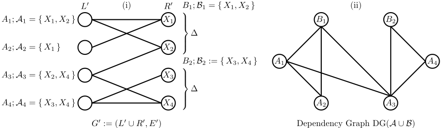
Bad Events. Intuitively, the definition of bad events needs to ensure that when all of them do not occur, the following two statements are true: (i) the selected vertices in the second phase satisfy the remaining demands; (ii) the maximum disagreement of the selected vertices in the second phase is O(log∆) · OPT. This motivates us to define two groups of bad events: performance bad events A and feasibility bad events B. The bad event in A is used to ensure that the selected vertices are able to achieve a good ratio. To this end, for each vertex in u ∈ L′ , we define a bad event Au stands for |NG′ (u) ∩ S2| > O(log ∆) · OPT, where NG′ (u) is a set of neighbors of vertex u in graph G′ . The bad event in B is used to ensure that the number of vertices in S2 satisfies the remaining demand requirement. To this end, we group vertices in R′ into several subgroups according to the index of vertices such that each subgraph consists of ∆ vertices from R′ . Let D1, . . . ,Dℓ ⊆ R′ be these subgroups. Note that the size of the last subgroup Dℓ may be smaller than ∆. For each subgroup Di, i ∈ [ℓ - 1], we define a bad event Bi to represent |Di ∩ S2| < ∑u∈Di x∗u . Intuitively, this inequality requires that the number of selected vertices in Di is at least ∑u∈Di x∗u . For the last subgroup Dℓ, we shall not define a bad event if ∑u∈Dℓ (x∗u + 1∆ ) < 1; otherwise, Dℓ also has a bad event Bℓ. Intuitively, if Dℓ has no bad event, then ∑u∈Dℓ x∗u is small; thus, we will not create a big demand gap in the case where no vertex is selected from Dℓ. The reason why we need to distinguish the last subgroup is that we have to upper bound the probability that a bad event happens; its meaning will be clear in the proof of Lemma 10. See Definition 1 for the formal definition of the bad events. An example can be found in Figure 1.

Definition 1 (Bad Events). The bad event set A∪B consists of two types of bad events, where bad events A and B are called performance bad events (P-BE) and feasibility bad events (FBE), respectively.

(P-BE). For each vertex u ∈ L′ , we have a bad event Au in A. Define Au ⊆ X as a subset of random variables, each of which corresponds to a vertex in NG′ (u). We say Au occurs if: ∑i∈Au Xi ≥ 8 · ln(2e∆2 ) · (T ∗ + 1).

(F-BE). For each subgroup Dj, j ∈ [ℓ - 1], we have a bad event in B. The last subgraph Dℓ has a bad event if ∑u∈Dℓ (x∗u + 1∆ ) < 1; otherwise, Dℓ does not have a bad event. For each bad event Bj ∈ B, define Bj ⊆ X as a subset of random variables, each of which corresponds to a vertex in Dj. Say Bj occurs if: ∑i∈Bj Xi < ∑u∈Dj x∗u .

Let DG(A ∪ B) be the dependency graph of bad events in A and B. Lemma 6 gives a lower and upper bound of the maximum degree of DG(A ∪ B), which will be used later to connect our problem and Lov´asz Local Lemma.

Lemma 6. Let d be the maximum degree of the dependency graph DG(A∪B). Then, the following two inequalities hold: (i) d ≥ 1; (ii) d ≤ ∆2 , where ∆ is the maximum degree of the input bipartite graph.

In the following, we split the proof into two parts. In the first part (Part I), we focus on an assignment X of random variables in X that makes all bad events in A ∪ B not occur. We define S2 := {v ∈ R′ | Xv = 1 in X}. We show that S2 is a set of vertices that satisfies the claimed property. In the second part (Part II), we prove that Algorithm 2 is able to return such an assignment in the desired running time. The proofs in this part shall built on the Lov´asz Local Lemma stated in Lemma 3 and Lemma 4. The formal proofs of all these lemmas are shown in the full version [Li et al., 2025].

Part I: Properties of X and S2. We start with the correctness of the feasibility bad events' definition. Formally, we shall show that when all bad events in B do not occur, the demand gap is at most 1 at the end of the second phase.

Lemma 7. If Algorithm 2 enters the second phase and all bad events in B do not occur, then |S1| + |S2| ≥ k - 1.

Lemma 8 is mainly due to Lemma 5 and the definition of performance bad events.

Lemma 8. If Algorithm 2 enters the second phase but does not enter the third phase, and S2 is a solution that makes all bad events in A∪ B do not occur, then the following two claims are true: (i) |S1 ∪S2| ≥ k; (ii) ALG ≤ 12 · ln(2e∆2 ) · (OPT + 1).

Lemma 9 can be proved by Lemma 7 and Lemma 8, i.e., adding one more vertex increases the solution's value by at most 1.

Lemma 9. If Algorithm 2 enters the third phase and selects v∗ in the third phase. Assume that S2 is a solution that makes all bad events in A∪ B do not occur, then the following two claims are true: (i) S1 ∪S2 ∪{ v∗ } is a feasible solution; (ii) ALG ≤ 12 · ln(2e∆2 ) · (OPT + 2).

Part II: Finding X and S2. In this part, we upper bound the probability that a bad event occurs (Lemma 10 and Lemma 11). This shall prove that our bad events satisfy the condition of the Lov´asz Local Lemma (Lemma 4). And then, we use Lemma 3 to bound the running time of Algorithm 2.

Lemma 10. For each bad event Bi ∈ B, Pr[Bi occurs] ≤ 1 2ed , where d is the maximum degree of the dependency graph DG(A ∪ B).

Lemma 11. For each bad event Ai ∈ A, Pr[Ai occurs] ≤ 1 2ed , where d is the maximum degree of the dependency graph DG(A ∪ B).

Wrapping Up. Now, we are ready to prove Theorem 3.

Proof of Theorem 3. By Lemma 5, Lemma 8, and Lemma 9, we know that if Algorithm 2 returns a solution that makes all bad events not occur, then Algorithm 2 is a 12 ln(2e∆2 )(OPT + 2)-approximate algorithm. In the following, we show that Algorithm 2 finds a desired solution in polynomial time. By Lemma 10 and Lemma 11, we know that the probability that a bad event occurs is at most 1 2ed , where d is the maximum degree of the dependency graph. By Lemma 6, we know d ≥ 1. Hence, we have 1 2ed ≤ 1 e(d+1) . Thus, we have Pr[C occurs] ≤ 1 e(d+1) for any bad event C ∈ A∪B. We define p := 1 e(d+1) . Therefore, we have that e(d+1) · p = e(d+1) · 1 e(d+1) = 1 ≤ 1. Thus, the probability of defined bad events satisfies the condition of Lemma 4.

Since Lemma 3 implies Lemma 4 by setting xC = 1 d+1 for each bad event C ∈ A ∪ B, then Algorithm 2 finds a solution that makes all bad events not occur in expected time at most ∑C∈A∪B xC 1-xC = (1+ 1d ) · |A∪B| by Lemma 3. Recall that |L| = n and |R| = m. By Definition 1, we have |A| ≤ n and |B| ≤ ⌈ m∆ ⌉ ≤ m. By Lemma 6, we have 1 ≤ d ≤ ∆2 . Thus, (1+ 1d ) · |A∪B| is poly(n,m). Hence, the expected running time of Algorithm 2 is in poly(n), where n is the number of vertices in the input bipartite graph.

5 Conclusion

We study the fair k-set selection problem where we aim to select k sets from a given set system such that the maximum (weighted) occurrence times that an element appears in these k selected sets are minimized. Given a bipartite graph G := (L∪R, E), our problem is equivalent to selecting k vertices from R such that the maximum (weighted) number of selected neighbors of vertices in L is minimized. We demonstrate that the problem is NP-hard when the maximum degree ∆ = 3, and then we give a simple optimal algorithm for the ∆ = 2 case. For the laminar family case, we show that the problem is also in P. We give three LP-rounding algorithms that are logarithmic approximate for general bipartite graphs and bipartite graphs with a maximum degree ∆.

This work points out many interesting directions. Firstly, it would be interesting to see whether the approximation can be further improved. This may need a more involved LP formulation. In particular, it would be interesting to see whether the problem admits an Ω( logn log logn ) lower bound. Secondly, considering a more general case is interesting where we additionally require that the selected vertices form a base of some matroid. The pipage rounding still works for this case, but it is not clear whether an O(log∆)-approximate exists.

Acknowledgements

Chenyang Xu is supported by the National Natural Science Foundation of China (No. 62302166), the National Key Research Project of China under Grant No. 2023YFA1009402, and the Key Laboratory of Interdisciplinary Research of Computation and Economics (SUFE), Ministry of Education. Shi Li is supported by the State Key Laboratory for Novel Software Technology and the New Cornerstone Science Laboratory. We thank the anonymous reviewers for their valuable comments.

Contribution Statement

All authors in the paper have equal contributions and are corresponding authors, and thus, it is ordered alphabetically.