Iterated Belief Change as Learning

1 Introduction

Belief Change Theory [Alchourrón et al., 1985; Gärdenfors, 1988; Katsuno and Mendelzon, 1991] provides a principled framework for modifying an agent's current beliefs in response to new information. Iterated belief revision [Darwiche and Pearl, 1997; Jin and Thielscher, 2007; Booth and Meyer, 2006] extends this framework to accommodate sequences of new information, addressing the challenge of revising an agent's beliefs over time. In both cases, the ultimate goal is to improve the agent's beliefs to better reflect the real world. While the methodologies of these two approaches differ, their objective aligns with that of Machine Learning (ML): deriving an accurate approximation of the real world from data.

Despite this conceptual similarity, connections between Belief Change Theory and ML remain largely unexplored, apart from a few notable contributions in philosophical logic [Kelly, 1998; Kelly, 2014; Baltag et al., 2011; Baltag et al., 2019], inductive logic programming [Wrobel, 1994; Pagnucco and Rajaratnam, 2005], and computational learning theory [Goldsmith et al., 2004].

A major difference is that primacy of update, which requires fully adopting new information after each revision, is a key principle in belief revision. However, this principle is incompatible with typical ML scenarios involving noisy data, as it leads to substantial changes in the agent's epistemic state at each learning step.

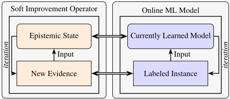
Improvement operators [Konieczny and Pino Pérez, 2008; Konieczny et al., 2010], which generalize iterated belief revision, relax the primacy of update. Soft improvement operators [Konieczny and Pino Pérez, 2008], in particular, allow incremental changes that better reflect the iterative nature of learning. When the same information is encountered again, its reliability is slightly adjusted. This mirrors the behavior of online ML methods for classification, where each labeled example causes gradual changes to the estimated probabilities of the classes.

Figure 1 illustrates this analogy. Most ML methods also adjust examples similar to the labeled example, those "near" the observed instance. A comparable mechanism can be introduced into the iterated belief change framework: both the observed example and its neighbors can have their reliability updated through an improvement operator.

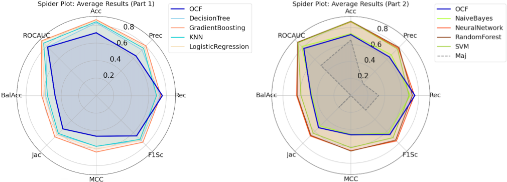
This paper focuses on binary classification and shows that improvement-based models built this way deliver reasonable learning performance. We compare them to standard ML methods on benchmark datasets. Results show the improvement-based model slightly outperforms Naive Bayes and achieves better recall than most existing methods. Thus, soft improvement operators offer a promising new approach to learning from examples.

Although an initial exploration, this connection is important for both KR and ML communities. It links two fundamentally different tasks - belief revision and supervised learning - with distinct goals and methods. From the ML side, this work opens the way to learning models that emphasize interpretability and offer strong guarantees linking the model to the data. These properties are crucial for trustworthy AI but often lacking in current ML models. If rationality principles are established, they could serve as safeguards to ensure the model evolves correctly with new evidence.

The proofs and code used to retrieve datasets and conduct experiments are available in [Schwind et al., 2025].

2 Preliminaries

We assume the reader familiar with basics of ML, including standard models (see, e.g., [Shalev-Shwartz and Ben-David, 2014] for an introduction). In this work, the focus is laid on tabular datasets, where instances are represented as vectors of Boolean features, aligning with many learning methods, especially in data mining. Such a Boolean encoding aids normalization, which often improves model performance. Although features in tabular data are usually not Boolean in essence, they can be converted accordingly. Categorical features are transformed via standard one-hot encoding, creating a Boolean feature for each domain value. Numerical features are converted by selecting thresholds within their domain to produce Boolean features. These thresholds are chosen by analyzing the data distribution (e.g., percentiles) or by optimizing split metrics like Gini impurity or entropy, as commonly done in tree-based models such as decision trees, random forests, and boosted trees.

Let L be a propositional language built from a finite set of propositional variables P, standard logical connectives, and the Boolean constants ⊥ (false) and ⊤ (true). A world on P is a mapping from P to {0, 1}, and Ω denotes the set of all such worlds. A world ω satisfies a formula ϕ if ω makes ϕ true; the set of such worlds is denoted by [ϕ]. A formula is consistent if [ϕ] ̸= ∅, and it is complete if [ϕ] = {ω} for some ω ∈ Ω. The symbol |= denotes logical entailment, and ≡ logical equivalence: ϕ |= ψ iff [ϕ] ⊆ [ψ], and ϕ ≡ ψ iff [ϕ] = [ψ].

Iterated Belief Change provides a principled framework for modeling how a rational agent's beliefs evolve with successive pieces of evidence. An agent's belief state, called an epistemic state, includes both the agent's current beliefs and conditional information that guides how beliefs should change in response to new inputs. Formally, an epistemic state can be any object Ψ, from which the agent's current beliefs are extracted via a mapping Bel, such that Bel(Ψ) ∈ L [Darwiche and Pearl, 1997]. An epistemic space is then a tuple E = 〈E, Bel〉, where E is the set of all epistemic states in the space [Schwind et al., 2022].

A standard example of epistemic space is built with Ordinal Conditional Functions (OCFs) [Spohn, 1988; Williams, 1995]. An OCF κ is a mapping associating each world with a non-negative integer 1 such that κ(ω) = 0 for some world ω.

Definition 1 (OCF epistemic space). The OCF epistemic space is the epistemic space Eocf = 〈Eocf , Belocf 〉 where:

• Eocf is the set of all OCFs over Ω;
• Belocf is the mapping associating each OCF κ from Eocf with a formula ψ ∈ L such that [ψ] = {ω ∈ Ω | κ(ω) = 0}.

Given an epistemic space E = 〈E,Bel〉, an iterated belief change operator ◦ on E is a mapping associating each epistemic state Ψ ∈ E and each formula µ ∈ L with a new epistemic state Ψ ◦ µ ∈ E, i.e., ◦ : E × L → E.

1 In the original definition OCFs are defined on ordinals [Spohn, 1988], but here, as in most cases, integers suffice.

Improvement operators [Konieczny and Pino Pérez, 2008; Konieczny et al., 2010; Medina Grespan and Pino Pérez, 2013] generalize iterated revision operators [Darwiche and Pearl, 1997] by dropping the success postulate (R*1), which requires the revised beliefs to entail the input formula. They are defined by nine rationality principles (I1)-(I9) (see [Konieczny and Pino Pérez, 2008; Konieczny et al., 2010] for details). We recall only the weak primacy of update:

This property states that after receiving α repeatedly, it eventually becomes believed.

We now introduce a simple example of an improvement operator defined over the OCF epistemic space:

Definition 2 (Basic shifting operator ◦+1). The basic shifting operator ◦+1 on Eocf is defined for any OCF κ and formula α by κ′ = κ ◦+1 α, where for each world ω ∈ Ω:

where x = 0 if Bel(κ) ∧ α ̸|= ⊥, and x = 1 otherwise.

Upon receiving new input α, the improvement operator ◦+1 adjusts κ by increasing the value of worlds ω ∈ [¬α] by 1 (i.e., κ′ (ω) = κ(ω) + 1), while leaving κ(ω) unchanged for worlds ω ∈ [α]. A normalization step (-x) then ensures min{κ′ (ω) | ω ∈ Ω} = 0, as required by the definition of an OCF. This operator resembles Spohn's n-conditionalization [Spohn, 1988], except n here depends on the prior plausibility of α (shifted by -1). It also relates to the one-improvement operator in [Konieczny and Pino Pérez, 2008].

2.1 Morphological Dilation and Erosion

An essential component for defining our learning operators is the notion of formula dilation and, dually, formula erosion [Bloch and Lang, 2002]. Both rely on a neighborhood B, which is a mapping associating each world ω ∈ Ω with a set of worlds Bω ⊆ Ω such that (i) ω ∈ Bω, and (ii) ω′ ∈ Bω implies that ω ∈ Bω′ , for all worlds ω, ω′ ∈ Ω.

A neighborhood B induces a dilation δB and an erosion ϵB, both mappings from formulas to formulas, defined for each ϕ ∈ L as follows:

• [δB(ϕ)] = {ω ∈ Ω | Bω ∩ [ϕ] ̸= ∅}
• [ϵB(ϕ)] = {ω ∈ Ω | Bω ⊆ [ϕ]}

For k ≥ 0, the k-dilation δkB (ϕ) and k-erosion ϵkB (ϕ) are defined inductively as follows: δ0B (ϕ) = ϕ, and δkB (ϕ) = δB(δk-1 B (ϕ)) for k > 0. Similarly, ϵ0B (ϕ) = ϕ, and ϵkB (ϕ) = ϵB(ϵk-1 B (ϕ)) for k > 0.

Neighborhoods can be derived from various similarity or distance measures on Boolean vectors (see [Choi et al., 2009] for an overview of such measures). In the present setting, the neighborhood Bω of each world ω depends solely on ω and need not be defined uniformly over Ω. Leveraging such instance-specific neighborhoods is known to be beneficial from a learning perspective [Ye et al., 2016].

3 FromEpistemic Spaces to Classifier Spaces

In this section, we formalize the change operation underlying the learning process of a binary classifier, drawing on the framework of iterated belief change introduced earlier.

The binary classification task consists in predicting whether a given instance is a member of some target class or concept. We assume that each instance is described by a vector of values associating each feature xi from a given finite and fixed set X with a value. We focus on binarized instance descriptions, so that the feature set X consists of a set of binary features. An instance can be associated with an output (1 or 0), characterizing whether the instance is predicted as positive or negative.

We represent each binary feature as a propositional variable, so that the feature set X corresponds to the set PX = {x1, . . . , xn}. A world over PX is called an instance description. Let ΩX be the set of all such instance descriptions, i.e., all worlds over PX, and let LX denote the propositional language generated from PX using the standard connectives. Each formula ϕ ∈ LX can represent a concept predicted by a binary classifier: an instance description ωX ∈ ΩX satisfies ϕ if and only if it is classified as positive. This modeling approach follows that of [Schwind et al., 2023].

To represent labeled data, as in training examples, we extend PX with an additional output (class) variable y indicating whether an instance is positive (1) or negative (0). Formally, we define P = PX ∪ {y}, with y /∈ PX. A world ω over P is called a labeled instance, and Ω denotes the set of all such labeled instances. A labeled instance ω is positive if ω(y) = 1 and negative if ω(y) = 0.

For any labeled instance ω ∈ Ω, its feature description (i.e., the corresponding world over PX) is denoted ωX. The complete formula ϕω ∈ L such that [ϕω] = {ω} is called a training instance, with ω its associated labeled instance. Let Lc denote the set of all such training instances. A dataset D is defined as a finite sequence of training instances: D = (ϕsω )1≤s≤m, and D denotes the set of all possible datasets.

To model binary classifiers, we move beyond treating a classifier as a static propositional formula (as in [Schwind et al., 2023]) and instead adopt a dynamic perspective that captures the learning process itself. This shift mirrors the move from one-step belief change - where an agent's epistemic state is represented by a single propositional formula [Katsuno and Mendelzon, 1991] - to iterated belief change, where epistemic states have a richer structure and yield formulas via the mapping Bel [Darwiche and Pearl, 1997].

Similarly, modeling the evolution of a classifier during learning requires a more expressive framework. To address this, the notion of an epistemic state is lifted to that of a binary classifier state. Likewise, the mapping Bel, which assigns each epistemic state with a propositional formula representing the agent's beliefs, is lifted to a mapping Pos, which assigns each classifier state with a formula characterizing the concept it predicts. The pair consisting of a classifier state and the mapping Pos thus forms a classifier space, in direct analogy with an epistemic space. The distinct notation Pos highlights the shift in perspective: from beliefs held by an agent to predictions made by a classifier. Formally:

Definition 3 (Classifier space). A classifier space is a tuple E = 〈E, Pos〉, where E is a set of binary classifiers and Pos is a mapping from E to LX.

Thus, the formula Pos(Ψ) represents the concept predicted byΨ: the set [Pos(Ψ)] contains the instance descriptions that Ψ classifies as positive, while [¬Pos(Ψ)] contains those classified as negative. Note that Pos(Ψ) is not required to be a consistent formula, i.e., [Pos(Ψ)] may be empty.

Standard epistemic spaces used for defining improvement operators can be directly adapted to build classifier spaces. Given an epistemic space E = 〈E, Bel〉, one can construct a classifier space E ′ = 〈E, Pos〉 by simply setting Pos = Bel. However, more meaningful examples of classifier spaces will be introduced in the next section.

Based on classifier spaces, we define an (online) learning operator:

Definition 4 (Learning operator). Let E = 〈E, Pos〉 be a classifier space. A learning operator ⊙ on E is a mapping ⊙ : E × Lc → E.

Thus, ⊙ specifies how a classifier Ψ ∈ E changes upon receiving a training instance ϕω ∈ Lc , yielding a new classifier Ψ⊙ ϕω. The framework is general enough to capture any binary classifier and online learning process, assuming binarized training data.

We now have the tools to define what we call a learning framework, representing a full learning process:

Definition 5 (Learning framework). A learning framework is a pair (Ψ∗,⊙), where Ψ∗ ∈ E is a binary classifier called the anchor, and ⊙ is a learning operator on E = 〈E, Pos〉.

The anchor Ψ∗ serves as the initial classifier state, providing the starting point for learning. Thus, a learning framework is fully determined by two components: the learning operator ⊙, which governs how classifiers evolve, and the anchor Ψ∗, which sets the initial state. Given a learning framework (Ψ∗,⊙) and a training dataset D ∈ D, the resulting learned classifier, denoted Ψ∗ ⊙D, is defined inductively by: 2

• Ψ∗ ⊙∅ = Ψ∗
• Ψ∗ ⊙ (D ⊔ (ϕω)) = (Ψ∗ ⊙ D) ⊙ ϕω

The choice of anchor depends on the context: it may be a classifier pre-trained on prior data, an untrained classifier (e.g., initialized as trivially positive, Pos(Ψ∗) ≡ ⊤, or negative, Pos(Ψ∗) ≡ ⊥), or a random element from E.

This formalization captures the iterative nature of online binary classifier learning and leads into the next section, where we introduce a specific class of learning frameworks.

4 Improvement-Based Learning

In this section, we introduce a concrete class of improvementbased learning operators. These operators are defined on a classifier space that extends the OCF epistemic space. In this space, each binary classifier is represented as a tuple (D, κ, τ), consisting of a training dataset D, an OCF κ, and a threshold τ ∈ R. Such classifiers are called TOCFS:

2⊔ denotes vector concatenation.

Definition 6 (TOCF classifier space). The TOCF classifier space is the tuple Etocf = 〈Etocf , Postocf 〉, where:

• Etocf = D×Eocf ×R is the set of all TOCFS
• Postocf is the mapping associating each TOCF (D, κ, τ) ∈ Etocf with a formula ψ ∈ LX such that [ψ] = {ω ∈ ΩX | κ(ω) ≤ τ}.

In this setting, a binary classifier is thus a TOCF Ψ = (D, κ, τ ).

The dataset D represents the training data used to construct Ψ. The OCF κ assigns a value to each instance description ωX ∈ ΩX, with lower values indicating greater plausibility that the instance is classified as positive by Ψ. The threshold τ specifies the classification boundary: an instance ωX is classified as positive (i.e., ωX ∈ [Pos(Ψ)]) if κ(ωX) ≤ τ, and as negative otherwise.

Our concrete class of learning operators is defined on the TOCF classifier space. Every operator in this class is specified by the following components:

• an improvement operator ◦ on the OCF epistemic space,
• a neighborhood B on ΩX (see Sec. 2.1), used to characterize formula dilation and erosion, and
• a performance metric m : N4 →R.

In a nutshell, the improvement operator ◦ and the neighborhood B are used together to adjust the plausibility of worlds in the underlying OCF κ of a TOCF Ψ = (D, κ, τ), while the performance metric m sets the threshold τ that best separates predicted positive and negative instances.

Given an improvement operator ◦, a neighborhood B, and a performance metric m, we denote the corresponding learning operator by ⊙(◦,B,m). Then, for any TOCF Ψ = (D, κ, τ ) and any training instance ϕω, the resulting TOCF Ψ′ = (D′ , κ′ , τ ′ ) = Ψ⊙(◦,B,m) ϕω is defined as follows.

First, we set D′ = D⊔(ϕω), that is, we augment the current training dataset by including the new instance ϕω.

Second, we build the new OCF κ′ using the improvement operator ◦ and the neighborhood B. This construction proceeds differently depending on whether the training instance ϕω is labeled as positive or negative.

Learning froma positive instance. If the training instance ϕω satisfies ϕω |= y, the process unfolds as follows. Let ϕωX ∈ LcX be the formula describing the instance (recall that ωX denotes its feature description). We begin by applying the improvement operator ◦ to ϕωX in κ, yielding κ ◦ ϕωX . We then continue this process iteratively on successive dilations of ϕωX : first on δB(ϕωX ), then on δ2B (ϕωX ), and so on, until reaching a fixed point.

Semantically, this process increases the plausibility of ω in κ, followed by an increase in the plausibility of its neighborhood, and then of neighborhoods of neighborhoods, so that the increase in plausibility assigned to a world becomes smaller as its distance from ω grows. Worlds that are not reachable from ω (that is, those not included in any dilation δkB (ϕωX ) for any k) remain unaffected; their plausibility in κ stays the same.

Formally, when ϕω |= y, we define the resulting OCF as κ′ = κ ·+ ϕωX = κ ·n+ ϕωX , where κ ·n+ ϕωX is inductively defined as follows:

• κ ·0+ ϕωX = κ,

Learning from a negative instance. Conversely, when the training instance is negative (ϕω |= ¬y), the process targets ¬ϕωX and its successive erosions: ϵB(¬ϕωX ), ϵ2B (¬ϕωX ), and so on. At each step, plausibility is increased for the worlds satisfying the current erosion, continuing until reaching a fixed point (or stopping just before if the fixed point is an inconsistent formula). Semantically, this increases the plausibility of worlds that are farther from ωX under B, with the increase being greater the farther the world is. The world ωX itself remains unaffected. Formally, we define κ′ = κ ·- ϕωX = κ ·n- ϕωX , where κ ·n- ϕωX is defined inductively as follows:

• κ ·0- ϕωX = κ,

An alternative would be to handle negative instances using a decrement operator applied to ϕωX and its successive dilations, mirroring the treatment of positive instances. While such decrement operators have been proposed [Sauerwald and Beierle, 2019], we do not adopt them here because, unlike the well-established duality between erosion and dilation, no formal duality exists between improvement and decrement operators. By relying on erosion and dilation - dual operations defined over a single neighborhood B - we maintain a unified learning mechanism using the same improvement operator for both positive and negative instances.

Given the distinction outlined above between learning from positive and negative instances, the new OCF is defined as:

Third, we define the threshold τ ′ , which acts as the "optimal separator." Recall that τ ′ partitions the space of instance descriptions such that instances with plausibility less than or equal to τ ′ are classified as positive, and those with plausibility greater than τ ′ are classified as negative. According to Def. 6, this corresponds to [Pos(Ψ′ )] = {ωX | κ′ (ωX) ≤ τ ′ }. We aim to select τ ′ so as to optimize performance over the dataset D′ , using the performance metric m.

For any candidate threshold τ ∈ N, we compute a confusion matrix cm(τ ) = (tp, fp, tn, fn) as follows:

• tp = {|ωX ∈ ΩX | ϕω ∈ D′ , ϕω |= y, κ′ (ωX) ≤ τ|}
• fp = {|ωX ∈ ΩX | ϕω ∈ D′ , ϕω |= ¬y, κ′ (ωX) ≤ τ|}

• fn = {|ωX ∈ ΩX | ϕω ∈ D′ , ϕω |= y, κ′ (ωX) > τ|}

The final threshold τ ′ is selected as the median among all integer thresholds τ ∈ [0, up] having the maximum score m(cm(τ)), where up = argmax({κ′ (ωX) | ωX ∈ ΩX}): 3

3 It suffices to search in [0, up]: thresholds τ < 0 yield the same confusion matrix as τ = 0, and τ > up as τ = up.

Having characterized both the new OCF κ′ and the threshold τ ′ , we now summarize the complete definition of the improvement-based learning operator ⊙(◦,B,m):

Definition 7 (Improvement-based learning operator ⊙(◦,B,m)). Let ◦ be an improvement operator, B be a neighborhood, and m be a performance metric. The improvement-based learning operator induced by ◦, B, and m, and denoted by ⊙(◦,B,m), is defined on the TOCF classifier space Etocf as follows. For each binary classifier (D, κ, τ) ∈ Etocf and each training instance ϕω ∈ Lc , we define (D, κ, τ ) ⊙(◦,B,m) ϕω = (D′ , κ′ , τ ′ ), where:

To define the "full" learning framework (cf. Def. 5), we must specify an anchor serving as an initial state. We choose Ψ⊤∗ = (∅, κ⊤, 0), where κ⊤ is the constant OCF assigning 0 to every world ωX ∈ ΩX. Hence, the full improvement-based learning framework is given by the pair (Ψ⊤∗ , ⊙(◦,B,m)).

5 An Instantiated Learning Operator

We now present a concrete instantiation of an improvementbased learning operator, ⊙(◦+1,BH ,mba). This operator is fully defined by the following choices:

• ◦+1, the basic shifting improvement operator (cf. Sec. 2)
• BH , that defines pairs of worlds as direct neighbors when they differ on at most one variable, i.e., for each ωX ∈ ΩX:

• mba, the balanced accuracy metric, defined for each confusion matrix (tp, fp, tn, fn) as:

The choice of balanced accuracy is illustrative rather than principled. Nonetheless, it is particularly appropriate for imbalanced datasets, where one class outweighs the other. By giving equal importance to the true positive rate and the true negative rate, balanced accuracy ensures a more equitable evaluation of classifier performance across both classes.

Representation of (Ψ⊤∗ ,⊙(◦+1,BH ,mba)). We now show that, in this specific learning framework, both a training algorithm and an inference algorithm (predicting the label of any instance ωX ∈ ΩX from a trained classifier) can be designed. Both algorithms run in polynomial time with respect to the number of training instances and the number of features.

Given an instance description ωX ∈ ΩX, let ωX ∈ ΩX be defined as ωX(xi) = 1 - ωX(xi), for each xi ∈ PX. Let dH : ΩX × ΩX → N be the Hamming distance between instance descriptions, i.e., for all ωX, ω′X ∈ ΩX,

We extend the Hamming distance to define a distance between any instance description ω′X and dataset D as dH(ω′X, ∅) = 0, and if D ̸= ∅:

On the other hand, given any dataset D, let ωDX ∈ ΩX be any instance description such that for each xi ∈ PX:

where D1 (xi) = |{ϕω ∈ D | ϕω |= y iff ω(xi) = 1}| and D0 (xi) = m-D1 (xi) (recall that m is the number of training instances fromD.)

We can show that such an instance description ωDX is one of the "closest" instance description to the dataset D in terms of Hamming distance: 4

Lemma 1. For each dataset D ∈ D and each instance description ωX ∈ ΩX, we have dH(ωDX, D) ≤ dH(ωX, D).

Then, we can show that for each instance description ωX ∈ ΩX the value κ(ωX) can always be characterized via computations of Hamming distances to the currently trained dataset:

Proposition 1. For each TOCF Ψ = (D, κ, τ) and each instance description ωX ∈ ΩX, we have that:

This has several important implications for our learning framework (Ψ⊤∗ ,⊙(◦+1,BH ,mba)) in terms of computational complexity. Recalling that n is the size of the feature set and m is the number of training instances from D, we have:

Proposition 2. Let D ∈ D, and let Ψ⊤∗ ⊙(◦+1,BH ,mba) D = Ψ = (D, κ, τ ).

1. τ can be computed in time O(n · m2 )
2. given (D, τ), for each ωX ∈ ΩX, deciding whether ωX ∈ [Pos(Ψ)] can be done in time O(n · m)

As a consequence of Proposition 2, in the learning framework (Ψ⊤∗ ,⊙(◦+1,BH ,mba)), we obtain both a learning algorithm (the computation of τ) and an inference algorithm (the prediction for any instance ωX ∈ ΩX given (D, τ)) that run in polynomial time with respect to the number of training instances and the number of features (Proposition 2.1 and 2.2, respectively). Since inference can be performed in polynomial time from (D, τ) alone, the learned classifier (D, κ, τ) is fully characterized by (D, τ), i.e., the OCF κ is not needed.

Another noteworthy property of this learning framework is its robustness to dataset permutations. Given any dataset D = (ϕsω )1≤s≤m, let Dπ = (ϕπ(s) ω )1≤s≤m denote the dataset obtained by applying a permutation π : {1, . . . ,m} → {1, . . . ,m}:

Proposition 3. For any permutation π : {1, . . . ,m} → {1, . . . , m} and any dataset D ∈ D,

4 All proofs are available online [Schwind et al., 2025].

In other words, the learned classifier is invariant under reordering of the training instances. This is significant, as many standard learning models, such as decision trees, random forests, and k-nearest neighbors (k-NN), may produce different outputs depending on the order in which the data is processed. This corresponds to the commutativity postulate for improvement operators [Schwind and Konieczny, 2020], which states that no piece of information should be treated as more important than another when the order of input carries no meaningful priority.

6 Experiments

Empirical protocol. We implemented in Python the improvement-based learning model ⊙(◦+1,BH ,mba) (simply denoted by ⊙ onward). Its predictive performance was compared against the following standard ML models (learned using the scikit-learn library [Pedregosa et al., 2011] and considering default parameters): Logistic Regression, Naive Bayes, Decision Tree, Gradient Boosting, KNN, Neural Network, Random Forest, and SVM. In addition, a trivial learning model (named Maj) always predicting the majority class (positive or negative) in the training dataset was considered as a baseline.

The evaluation considered a large set of performance metrics that are standard in ML: balanced accuracy, accuracy, F1 score, Jaccard index, Matthews correlation coefficient (MCC), precision, recall, and ROC-AUC (receiver operating characteristic area under the curve).

The experimental protocol involved selecting 58 binary classification datasets from the UCI repository, 5 with each dataset containing up to 12,684 instances and up to 1,203 numerical or categorical features. A 10-fold cross-validation has been conducted: each dataset was split into ten random samplings, with a 90%/10% division for training and test sets. Missing values in the data were imputed by filling each numerical feature with the mean value from the dataset and each categorical feature with the most frequent value. The datasets were then standardized using a standard scaler.

5 https://archive.ics.uci.edu/datasets/

For our learning framework ⊙, numerical attributes were further re-scaled linearly to the interval [0, 10] with integer values, while categorical attributes were left unchanged. For these experiments, binarizing the features was not mandatory: instead, we used a modified weighted Hamming distance between instance descriptions d′H (ωX, ω′X). This was made only for convenience as this is equivalent in terms of performance and computational complexity to binarizing all datasets in such a way to ensure that dH = d′H .

Empirical results. We did an extensive comparative analysis which is visualized through various plots (the full set is available in [Schwind et al., 2025]). Box plots were generated for each metric, showing model performance across the 58 datasets, scatter plots compared the proposed model with each baseline, and spider plots have been used to compare the performance of all models for individual datasets and in an aggregate view. We present some of them hereafter.

The spider plots in Figure 2 show in a synthetic way the average predictive performances (over the 58 datasets) of the ten ML models learned for each of the ten families of models considered in our experiments and assessed for each of the eight metrics (our learning framework is simply named OCF in the figures). One can see that ⊙ outperforms the baseline Maj model (which is mandatory to be considered as a significant learning operator). It turns out that in practice⊙achieves performances that are similar to the ones of Naive Bayes. Finally, ⊙ performs slightly better than the other models when recall is used to measure the predictive performance. This is an important point since high recall is expected in applications where missing a positive case can be costly, such as in healthcare or when dealing with attack detection.

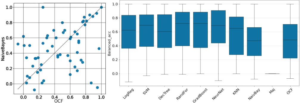
Focusing on the balanced accuracy metric, Figure 3 (left) presents a scatter plot for contrasting in a more precise way the predictive performances of ⊙ and Naive Bayes; and Figure 3 (right) presents boxplots representing the distributions of predictive performance achieved over all datasets by each of the ten ML models at hand. The results presented are coherent with those shown in Figure 2 (especially, the averaged balanced accuracy of ⊙ is slightly greater than the one of Naive Bayes and much better than the one of Maj).

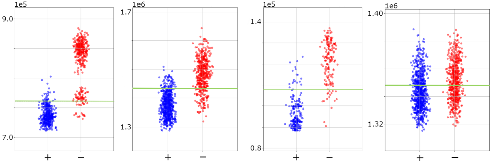
Additionally, Figure 4 showcases some learned classifers (D, κ, τ) for some test sets in some randomly chosen dataset samplings. Each figure depicts the value distribution of all κ(ωX) for each test instance ωX from the sampling, represented as a blue (resp. red) dot when ϕωX |= y (resp. ϕωX |= ¬y), and the green horizontal line corresponds to the threshold τ. It can be observed that the learned model separates quite accurately the positive instances from the negative ones for the first three samples, but clearly not for the last one (603-In-Vehicle Coupon Recommendation).

7 Conclusion

In this paper, we showed how improvement operators, grounded in Belief Change Theory, can give rise to a family of online learning models, and we have presented learning and inference algorithms designed for this family. We empirically evaluated the predictive performance of a specific model within this family using a range of datasets. While the results indicate that this simple model does not match the accuracy of more advanced models (e.g., neural nets), it performs comparably to all other methods in terms of recall. This makes it particularly suitable for applications where failing to detect positives is critical. Additionally, the model outperforms the trivial Majority class model and shows performance on par with Naive Bayes, suggesting a significant potential.

This work opens up several avenues for future research. Theoretically, the next step is to analyze the properties of learning operators derived from improvement operators. Empirically, we plan to explore and evaluate additional models within the proposed family. For instance, while the learning algorithm used in the experiments is based on Hamming distance, other distances, such as the Mahalanobis distance, could be explored [Mahalanobis, 1936]. Because it accounts for feature correlations which could be measured on the training set, the Mahalanobis distance appears as a valuable candidate for improving model performance at inference.

Acknowledgements

This work was supported in part by the following grants: JSPS KAKENHI Grant Numbers JP25K00375 and JP25K03190; JST CREST Grant Number JPMJCR22D3; the AI Chairs BE4musIA (ANR-20-CHIA-0028) and EXPEKCTATION (ANR-19-CHIA-0005-01) funded by the French National Research Agency.