Identifying Causal Mechanism Shifts Under Additive Models with Arbitrary Noise

1 Introduction

Causal discovery aims to uncover underlying causal relationships between variables of interest in observational data [Chen et al., 2024a; Zhang et al., 2024], which play a significant role in multiple disciplines such as genomic analysis [Xu et al., 2024] and epidemiology [Robins et al., 2000]. Numerous causal discovery algorithms have been proposed, including prominent methods such as PC [Spirtes et al., 2000] and GES [Meek, 1997]. More recently, methods based on properly defined Structural Causal Models (SCMs) have been proposed to distinguish the correct graph underlying the observational data, by adding additional assumptions on the functional class of the SCM [Hoyer et al., 2008; Zhang et al., 2021; Zhang et al., 2022].

In practice, the ultimate goal in many applications is not to recover the entire underlying DAG, but rather to detect the changes in the causal mechanisms among multiple related domains. For example, one application involves identifying the root causes of faults in large-scale manufacturing and industrial control systems [Bogatinovski et al., 2021]. Another important application lies in identifying differences in gene regulatory networks between healthy individuals and cancer patients. The key genes that explain these differences may provide valuable information on potential therapeutic targets for specific types of cancer [Hudson et al., 2009]. In these applications, compared with the size of the whole causal graph, the number of variables whose causal mechanisms change among domains tends to be relatively sparse. As a result, estimating causal graphs for each individual domain and subsequently detecting changes is inefficient and redundant. Therefore, it is of significant importance to develop a practical method for directly detecting changes in causal mechanisms across different environments.

Most existing methods for identifying causal mechanism shifts rely on restrictive assumptions within the functional class of the SCM, which can limit their applicability in realworld scenarios. For instance, both DCI [Wang et al., 2018] and the method proposed by [Varici et al., 2021] assume that the underlying SCM adheres to a linear ANM with Gaussian noise. To relax the linearity constraint, UT-IGSP [Squires et al., 2020] introduces a nonparametric approach for identifying intervention targets. However, this method depends on nonparametric conditional independence (CI) tests, which are computationally expensive and inefficient. More recently, iSCAN [Chen et al., 2024b] leverages the Jacobian of the score function of the mixture distribution to detect mechanism shifts. Despite its advancements, this approach imposes strict assumptions on the noise distribution in the ANM, which further restricts its applicability in practical scenarios.

Building on recent advancements in identifying causal relationships within multivariate ANMs with arbitrary noise distributions [Montagna et al., 2023], we propose a novel method for detecting shifts in causal mechanisms that is applicable to arbitrary noise distributions. Specifically, we establish a connection between the score function of the mixture distribution across environments and the identification of variables whose causal mechanisms shift under arbitrary noise distributions. Based on this theoretical insight, we develop a practical algorithm that iteratively detects common leaf variables across all environments and evaluates whether their causal mechanisms have shifted by leveraging the score function. In summary, our main contributions are as follows:

• We prove that the score function of the mixture distribution unveils information to detect mechanism shifts for the common leaf nodes, which does not rely on any structural assumptions on the individual DAGs or parametric assumptions on noise distributions.
• We propose an algorithm that iteratively selects a common leaf variable among the DAGs in different environments and evaluates whether such variable is shifted.
• We evaluate the performance and applicability of our method by extensive experiments on both synthetic and ovarian cancer datasets. The results demonstrate the superiority of our method.

The remainder of this paper is organized as follows: In Section 2, we list the previous works in related topics. In Section 3, we introduce the fundamental notions and background. In Section 4, we present our method for detecting shifted variables. In Section 5, we evaluate the performance of our algorithm on both synthetic and ovarian cancer datasets. In Section 6, we summarize the content of this paper.

2 RelatedWork

Mechanism Shifts Identification. In the past decade, various approaches have been proposed to identify mechanism changes across environments. [Zhao et al., 2014; Yuan et al., 2017; Liu et al., 2017] propose algorithms for directly detecting the changes by estimating the difference between two precision matrices. However, these methods are only suitable for undirected graphs. For directed graphs that provide more essential information, [Li et al., 2023] offers a potential approach to detect heterogeneous functional relationships between a variable Xj and its parents. However, the applicability of their method is limited, as it relies on the assumption of a common distribution for covariates across different environments. This assumption is potentially violated if the mechanism shifts have affected the ancestors of Xj. Additionally, DCI [Wang et al., 2018] estimates changes by testing the invariance of regression coefficients and noise variances, while [Varici et al., 2021] repeatedly identifies intervention sites in subsets of variables by comparing precision matrices, both of which are restricted to linear additive noise models (ANMs) with Gaussian noise. To address the linearity constraint, UT-IGSP [Squires et al., 2020] introduces a nonparametric method for identifying intervention targets. However, this approach relies on nonparametric conditional independence (CI) tests, which can be computationally expensive and inefficient. iSCAN [Chen et al., 2024b] detects shifts by leveraging the Jacobian of the score function of the mixture distribution. Nonetheless, this method assumes that the noise distribution in the ANM satisfies specific conditions.

Application. Identification of causal mechanism shifts has wide-ranging applications across numerous domains. In biology, understanding differences in gene regulatory networks across different populations in biological systems can provide crucial insights into disease mechanisms and potential therapeutic targets [Hudson et al., 2009; Pimanda et al., 2007]. Specially, in the analysis of EEG signals it is of interest to detect neurons or different brain regions that interact differently when the subject is performing different activities [Sanei and Chambers, 2013]. In economics, [Shi et al., 2020] apply a new method to detect shifts in Granger causality, uncovering structural breaks in the US money-income relationship. Another application area lies in fault detection in large-scale Internet of things and cloud applications [Bogatinovski et al., 2021]. Other examples include epidemiology [Robins et al., 2000], medicine [Plis et al., 2010], etc. These diverse applications highlight the importance of developing robust and efficient methods for causal mechanism shift detection.

ScoreMatching. Score matching, a recently developed parameter learning method, is particularly effective for highdimensional density models with intractable partition functions [Lyu, 2012; Ren et al., 2025]. Recent advancements have extended score matching to generative modeling, resulting in score-based generative models that achieve remarkable performance in image generation and other domains [Song and Ermon, 2019; Song et al., 2020]. This method has also been explored in causal discovery. For instance, SCORE [Rolland et al., 2022] leverages the Jacobian of the score function to identify the topological order in additive noise models (ANMs) with Gaussian noise. NoGAM [Montagna et al., 2023] builds on this by learning causal relations through regression on the score function, relaxing the noise distribution constraints of iSCAN. Additionally, score matching's ability to capture subtle distribution changes makes it valuable for detecting distribution shifts. For example, iSCAN [Chen et al., 2024b] uses the diagonal of the Jacobian of the score function to identify shifts in causal mechanisms.

3 Preliminaries and Background

In this section, we first introduce the notation and assumptions that will be used throughout the paper. We then conclude by formalizing the problem setting.

Definition 1 (Structural Causal Model (SCM)). Let V = {1, ..., d} be the vertices of a directed acyclic graph G, and X = {X1, ...,Xd} be a d-dim vector of random variables, in one-to-one correspondence with V . An SCMM= (X, f, PN) over d variables is a set of d structural equations with the same form:

where PAi ⊆ V \ {i} are the direct parents of vertex i in the underlying DAG of the SCM. PN is the joint distribution of noise terms N = {N1, ...,Nd} which are assumed to be jointly independent 1 .

1 Note that we assume there is no latent confounders.

Definition 2 (Causal Mechanism). Every SCM induces a joint distribution P(X) of X and admits the following factorization:

where P(Xi|XPAi ) is defined as the causal mechanism of Xi. Definition 3 (Independent Causal Mechanisms (ICM) Principle). A change in P(Xj|PAj) has no effect on and provides no information on P(Xk|PAk) for any k ̸= j.

Denote an underlying SCMM∗ with DAG structure G∗ and joint distribution P∗ (X) = ∏dj=1 P∗ (Xj |XPA∗j ). An environment arises from intervening causal mechanisms of a subset of X. Formally, we have the following definition.

Definition 4 (Environment). An environment Eh is derived from an underlying ANMM∗ = (X, f, PN) by applying interventions on an unknown subset I of variables X. According to the ICM Principle (Def. 3), then the new joint distribution Ph (X) can be factorized as follows:

where Ph (Xi|XPAhi ) is the causal mechanism after intervention. Here, we allow an intervention to modify the causal mechanism of a variable while optionally removing part of its direct parents, i.e., PAhi ⊆ PA∗i .

With Def. 4, we have the definition of the shifted variables.

Definition 5 (Shifted Variable). A shifted variable is a variable whose causal mechanism differs across different environments. Formally, variable Xi is a shifted variable, if there exists two environments Ea and Eb, such that

where Pa (Xi|PAai ) and Pb (Xi|PAbi ) denotes the causal mechanisms of Xi in environment Ea and Eb, respectively.

Definition 6 (Additive Noise Model (ANM)). An additive noise model M∗ is an SCM whose each structural equation has the following form:

where fi is referred to as the data generation function.

In this paper, we assume that all SCMs in different environments satisfy the ANMmodel. That is, intervention can modify function fi, parent PAi or noise distribution Ni. However, the new SCM after intervention still follows the ANM model. Next, we introduce a lemma from [Montagna et al., 2023] which serves as the basis of our approach.

Lemma 1. Given X be a d-dim random variables generated according to Def. 5 with underlying DAG G. Let p(x) be the pdf of X and s(x) = ∇ log p(x) be the corresponding score function. Denote Ri be the residual of Xi by regressing on X\{i}, and then obtain g(Ri) as the estimator for si(X) by regressing on Ri. ∀ Xi ∈ X, we have:

Lemma 1 provides a sufficient and necessary condition for detecting leaf nodes for those models generated according to ANM. Notably, it requires no specific parametric assumption on the noise distribution. Finally, to conclude this section, we formally define the whole problem.

Problemdefinition. GivenH datasetsX1 , ...,XH sampled from K different environments where Xk ∈ Rmh×d consists of mh independent and identically distributed samples from environment Eh, our task is to identify the shifted variables relative to H environments without any assumptions on the specific noise distribution in the ANM.

4 Method

In this section, we propose CMSI to identify mechanism shifts across environments, without any assumptions about the noise distribution in the ANM.

Let X be the row concatenation of all the datasets Xh , i.e., X = [(X1 )⊤ | · · · | (XH )⊤]⊤ ∈ Rm×d , where m = ∑Hh=1 mh. The pooled data X represents an aggregation of data sampled from H heterogeneous environments. To account for this aggregation, we introduce the probability mass wh ≜ mh m , which represents the probability that an observation belongs to the environment Eh, i.e., ∑Hh=1 wh = 1. Let Q(X) denote the distribution of the mixture data with density function q(x), i.e., q(x) = ∑Hh=1 whph (x). We use sh (x) ≜ ∇ log ph (x) to denote the score function of the joint distribution of environment h with density ph (x). Also, we use s(x) ≜ ∇log q(x) to denote the score function of the mixture distribution with density q(x).

4.1 Main Results

Inspired by Lemma 1 that identifies the leaf nodes in a single environment via the score function. In the sequel, we will show that the score function of the mixture distribution s(x) ≜ ∇log q(x) can help reveal causal mechanism shifts among different environments. Firstly, we make the following assumptions on the underlying SCM.

Condition 1 ([Peters et al., 2014]). Given a bivariate model Xi := Ni andXj := fj(Xi)+Nj, we call the SCMan identifiable bivariate ANM if the triple (fj, pNi , pNj ) does not solve the following differential equation for all pairs xi, xj with f ′ j (xi)g′′ (xj - fj(xi)) ̸= 0:

Here, f := fj, k := log pNi , g := log pNj . To improve readability, the arguments xj - fj(xi), xi and xi of g, k and f, respectively, have been removed.

Assumption 1. For all j ∈ V, i ∈ PAj and all sets S ⊆ V with PAj\{i} ⊆ S ⊆ NDj\{i, j}, there is an xS with pS(xS) > 0, s.t.

Algorithm 1 Regression the Score on Residual (ReSR)

Input: Dataset X.

Output: Estimator ˆ g(R) of the score s(X).

• 1: s(X) ← estimate the score function of X.
• 2: Ri ← residual by regressing Xi on X\{i}, ∀i ∈ V.
• 3: ˆ g(R) ← obtained by regressing s(X) on Ri, ∀i ∈ V.
• 4: return ˆ g(R).

satisfies Condition 1. In particular, we require the noise variables to have non-vanishing densities and the functions fj to be continuous and three times continuously differentiable.

Theorem 1. For all h ∈ [H], let Gh and ph (x) denote the underlying DAG structure and pdf of environment Eh, respectively, and let q(x) be the pdf of the mixture distribution of the H environments such that q(x) = ∑Hh=1 whph (x). Also, let s(x) = ∇log q(x) be the associated score function, Ri := Xi -EXi∼Q(Xi)[Xi|X\{i}], g∗ (Ri) := E[si(X)|Ri]. Then, under Assumption 1, we have: if l is a leaf in all DAGs Gh , then l is a shifted node if and only if:

except for the case that the causal functions are identical across environments, i.e. ∀h, h∗ ∈ [H], f h l = f h∗ l .

The proof of Theorem 1 is presented in the appendix. Theorem 1 provides an effective approach for detecting mechanism shifts for common leaf nodes. As the induced graph by M∗ is acyclic and each intervention will only optionally remove edges without adding some new edges, we can always find a common leaf node. Furthermore, after removing the common leaf node found, we can always find a new one, until the whole graph is empty. Consequently, all the shift nodes can be found in this procedure by Theorem 1.

The idea above is outlined in Alg. 2. Concretely, we first integrate the primary computational procedure of Lemma 1 into Alg. 1 as a component. In Alg. 1, to obtain the estimator ˆ g(R) of the score s(X), we first regress each variable Xi against the remaining variables X\{i} to get the residual Ri, and finally regress the score function s(X) against the residuals R. In Alg. 2, we first identify the leaf nodes of the underlying DAG for each environment based on Lemma 1 and then obtain the common leaf nodes L of all DAGs (Line 4-5). Subsequently, based on Theorem 1, we detect whether the common leaf nodes are shift nodes (Line 6-8). Repeat the above procedure until all variables have been detected (Line 9). Note that for each iteration, the common leaf nodes will not be involved in the subsequent identification of leaf nodes, regardless of whether they are shifted.

Computational Complexity. The computational complexity of both score function estimation and regression within a single environment Eh is O(dm3h ). In Alg. 2, the primary computational cost stems from the score function estimation on the pooled data X ∈ Rm×d and regression on X, each with a complexity of O(dm3 ). In the worst-case scenario, where only one node is removed per iteration, the algorithm requires at most d iterations. Therefore, the total computational complexity of Alg. 2 is O(d2m3 ).

Algorithm 2 Causal Mechanism Shifts Identification (CMSI)

Input: Dataset X1 , ..., XH .

Output: Estimated shifted variables set ˆI.

• 1: Initialization: ˆI = {},N = {1, ..., d}.
• 2: X = [(X1 )⊤| · · · | (XH )⊤]⊤ ∈ Rm×d .
• 3: while N = ∅ do
• 4: ˆ g(Rh ) ← ReSR(Xh ), ∀h ∈ [H].
• 5: L←∩h∈[H]{l | E[(sl(Xh ) - ˆ g(Rh l ))2 ] = 0, l ∈ V}.
• 6: ˆ g(R) ← ReSR(X).
• 7: ˆI ←ˆI ∪ {Xi | E[si(X) - ˆ g(Ri))2 ] ̸= 0, i ∈ L}.
• 8: remove Xh [:, L] and X[:, L], ∀h ∈ [H].
• 9: N ←N -{L}.
• 10: end while
• 11: return ˆI.

4.2 Practical Implementation

In this section, we present some practical implementation details of Alg. 2 used in the experiments.

Score Function Estimation. Given an environment E and its dataset X = {x1 , ..., xm} ∈ Rm×d . To estimate the corresponding score function s(x) = ∇log p(x), Stein's identity [Stein, 1972] provides an estimator using:

where h : Rd → Rd′ s.t. limx→∞h(x)p(x) = 0. In practice, we adopt a similar approach to the method in [Li and Turner, 2017] and present the estimator for the point-wise first-order partial derivative, corresponding to Eq. (10):

where H = (h(x1 ), . . . , h(xm)) ∈ Rd′×m, K = H⊤H, Kij = κ(xi , xj ) = h(xi )⊤h(xj ), ∇h = 1m ∑mk=1 ∇h(xk ), ⟨∇, K⟩ = mH⊤∇h, and η ≥ 0 is a regularization parameter. G ≡ (∇log p(x1 ), . . . ,∇log p(xm))⊤ ∈ Rm×d and ˆG is used to approximate G.

Regression. In both stages of regression in Alg. 1, we utilize kernel ridge regression due to its capability to model nonlinear relationships. To enhance computational efficiency, we implement kernel ridge regression with NVIDIA's cuML library from the RAPIDS AI open-source software suite. The regularization coefficient in the kernel ridge regression is set to α = 0.1, and we use the radial basis function (RBF) kernel with a width parameter of γ = 0.1.

Selection of Common Leaf. Before employing Theorem 1 to examine the shifted nodes, it is necessary to leverage Lemma 1 first to obtain the leaf nodes in each individual environment Eh and then deduce the common leaf nodes among all environments. Estimating E[(shi (X) - ˆ g(Rh i ))2 ] is performed by computing the Mean Squared Error (MSE) between the prediction ˆ s(Rh i ) and the ground truth si(Xh ), denoted as MSEhi . In practice, due to the limited number of samples, it is not feasible to select leaf nodes solely by MSEhi = 0 because MSEhi is susceptible to errors. Therefore, we first rank the nodes based on their individual MSEhi values in each environment Eh. Subsequently, we select the node with the minimum sum of ranks across all environments as the common leaf.

Selection of Shifted Variables. Based on X, the row concatenation of all datasets Xh , we compute the score function s(X) and its estimator ˆ s(R) based on the residuals R. Similarly to the selection of common leaf, the estimation of E [(si(X) - ˆ s(Ri))2 ] is performed by computing MSEi and limited samples can introduce errors in MSEi. Therefore, similar to [Chen et al., 2024b], we introduce the following statistic for each common leaf l:

The ratio MSEl minh MSEhl distinguishes between shifted and nonshifted common leaf nodes l. For shifted nodes, the ratio is large. For non-shifted nodes, the ratio is small, as MSEl converges to zero faster than MSEhl , supported by the larger dataset used for MSEl computation (Theorem 1). The small

ϵ in the denominator ensures numerical stability, e.g., 10-9 . We iteratively identify common leafs and calculate the value of this ratio for each common leaf. This process ultimately generates a dictionary where each key-value pair comprises a node index and its corresponding stat value. After sorting this dictionary in non-increasing order, we utilize the Python library kneed to find the knee point which is the point of maximum curvature in a curve. Finally, we selected the knee point as the boundary between shifted and non-shifted nodes.

5 Experiments

In this section, we illustrate the capability of our algorithm CMSI through extensive experiments on synthetic and realworld datasets. In Section 5.1, we evaluate the algorithm's ability to detect shifted variables on synthetic datasets, where the data generation function is characterized as a composite trigonometric function. In Section 5.2, we demonstrate the application of CMSI to real-world scenarios by experiments on an ovarian cancer dataset. Additionally, we provide additional experiments in the Appendix including: (1) Extended evaluations on shifted variable identification using the datagenerating functions of Section 5.1. (2) Identifying shifted variables when the data generation is generated by sampling Gaussian processes. (3) Identifying shifted variables when the underlying causal graph structures are different.

5.1 Synthetic Experiments

Basic Settings. We use the Erd¨os-R´enyi (ER) and ScaleFree (SF) graph models to generate random DAGs with d nodes (d ∈ {20, 30, 40, 50}) and kd edges (k ∈ {2, 4, 6, 8}). The default sample size in each environment equals 500.

Synthetic Dataset. Based on the generated causal graph and the additive noise model (noise ∈ {Gaussian(0, 1), Laplace(0, 1), Gumbel(0, 1), Exponential(1), Beta(1, 1), Gamma(0.5, 0.5)}), we construct the synthetic datasets. The non-shifted variables are generated by following additive noise model:

To generate the shifted variables, we first select a subset of non-root nodes as shifted nodes, based on a ratio r ∈ {0.15, 0.20, 0.25, 0.30}. For each shifted node, a single environment is randomly selected from all available environments to represent its shifted environment. The node does not undergo a shift in the remaining environments. (For example, consider a scenario with H = 3 environments, each containing d = 20 nodes. Using a ratio r = 0.2, we randomly select 4 non-root nodes as shifted nodes. Then, we randomly assign shifted node 1 to environment 2 for its shift, shifted node 2 to environment 1, and so on for the remaining shifted nodes. Each shifted node only exhibits a shift in its assigned environment.) For a shifted variable Xi ∈ I , we randomly select t direct parents ˜ PAi ⊆ PAi and then intervene in the relationships between ˜ PAi and Xi. Similar as [Chen et al., 2024b], the intervention is implemented by changing the generation

Basic Experimental Setup. We use F1 Score metric to evaluate the algorithm's ability to detect intervened variables. Experiments were conducted on a system equipped with an Intel Xeon(R) Platinum 8255C CPU and two NVIDIA GeForce RTX 2080 Ti GPUs.

Baselines. We compared the performance of CMSI against several baselines, which include: iSCAN [Chen et al., 2024b], CITE [Varici et al., 2021], Shapley [Budhathoki et al., 2021], DCI [Wang et al., 2018], UT-IGSP [Squires et al., 2020].

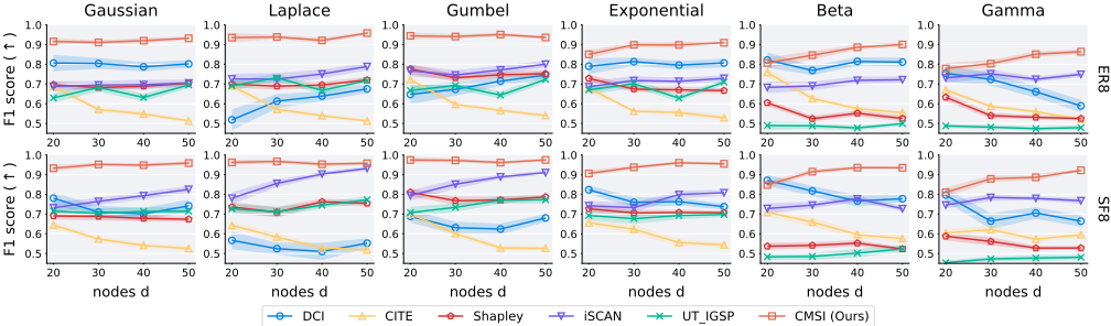
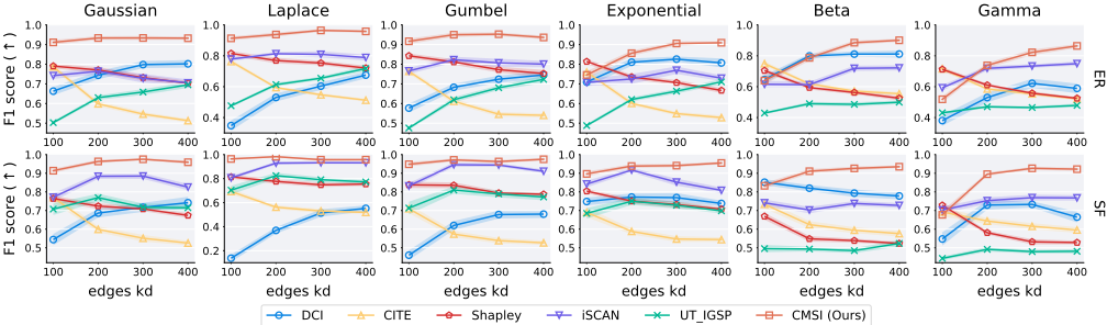
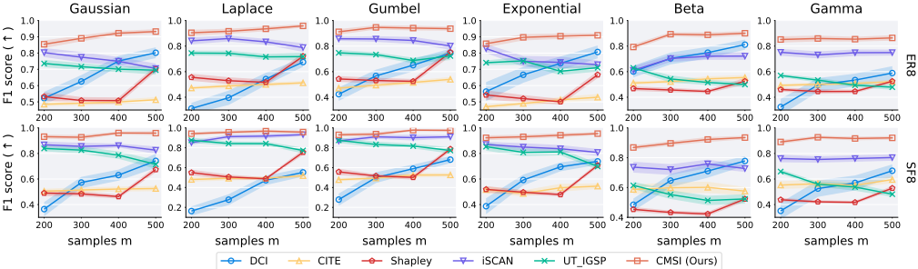
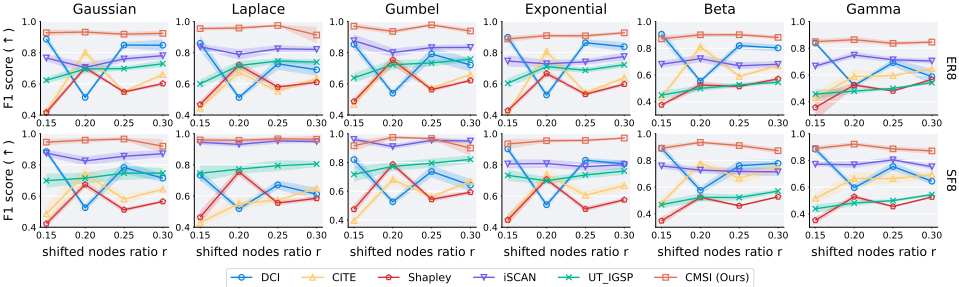
Overall Results Analysis. From Fig. 1∼4 we can see that CMSI consistently achieves state-of-the-art performance in terms of F1 score, compared with other well-performing baselines. In contrast, CITE and DCI exhibit the worst performance and the limitations are likely attributable to their inherent reliance on linearity restrictions on SCMs. In addition, CSMI exhibits the lowest standard deviation in general, indicating greater stability and reliability regardless of data variations. More significantly, considering different noise types, CMSI exhibits the best performance in most scenarios. This indicates that CMSI exhibits stronger robustness and generalization capabilities across different noise types.

Results w.r.t. number of nodes. Fig. 1 illustrates the results with d ∈ {20, 30, 40, 50} nodes and 8d edges. As the number of nodes increases, the performance of CMSI steadily improves under any noise conditions. In contrast, the performance of CITE decreases as the number of nodes increases. Furthermore, the trends exhibited by certain methods differ according to the type of noise present. For instance, DCI's performance improves with increasing node numbers under Laplace noise, but declines under Gamma noise.

Results w.r.t. number of edges. Fig. 2 displays the results with 50 nodes and 50k edges (k ∈ {2, 4, 6, 8}). The performance of CMSI consistently improves as the number of edges grows. This suggests that CMSI has stronger generalization abilities and excels at identifying shifted variables in denser causal graphs. A notable exception is the scenario presented in Fig. 2 where the edge count equal to 100 and the node count equal to 50. This represents the sparsest graph structure among all those tested with the largest number of nodes. Therefore, the lack of sufficient edge information (i.e., information about causal relationships) in this scenario hinders CMSI's ability to make accurate judgments, leading to slightly poorer performance. Nevertheless, numerous realworld applications (such as gene regulatory networks) involve dense causal graphs, ensuring the wide applicability of CMSI.

Results w.r.t. number of samples. Fig. 3 displays the results with 50 nodes, 400 edges and m samples (m ∈ {200, 300, 400, 500}). In general, an increase in the number of samples results in enhanced performance for algorithms, such as DCI. However, CMSI demonstrates stable performance across different sample sizes, indicating its ability to effectively acquire knowledge from the samples. This makes it suitable for shift detection in small-sample scenarios. In contrast, algorithms like DCI, Shapley, and CITE perform poorly with small sample sizes, while iSCAN and UT IGSP exhibit performance fluctuations as the sample size increases.

Results w.r.t. shifted nodes ratio. Fig. 4 displays the results with 50 nodes, 400 edges and shifted nodes ratio r ∈ {0.15, 0.20, 0.25, 0.30}). When the ratio r varies, the performance of DCI, and Shapley fluctuates significantly, but CMSI's performance remains stable and consistently the best. This suggests that CMSI can detect shifts in causal mechanisms under varying degrees of shift.

Additional Experiments. Due to space limitations, we leave more experiments in the Appendix. Additional experiments include 1) increasing the number of environments H ∈ [2, 3, 4, 5], 2) more flexible data generation processes using Gaussian process, 3) shifted variable identification with diverse causal structures. All results consistently imply that CMSI possesses greater general applicability than baseline methods. See the Appendix for more details.

5.2 Experiments on Ovarian Cancer Dataset

We evaluated CMSI on an ovarian cancer dataset [Tothill et al., 2008] that was previously analyzed by iSCAN [Chen et al., 2024b] and DCI [Wang et al., 2018]. This dataset was collected from patients with stage III or stage IV ovarian cancer and divided into two subsets based on survival duration. Based on these two subsets, CMSI identified the two most heavily intervened genes in the apoptosis pathway: BIRC3 and FAS. BIRC3 was also identified by iSCAN and DCI, but FAS was exclusively identified by CMSI as a highly intervened gene. In fact, BIRC3 is categorized as an inhibitor of apoptosis proteins (IAPs) , and the changes in BIRC3 expression levels induced by intervention affect the survival time of ovarian cancer patients [Hu et al., 2019]. In addition, FAS is highly expressed in ovarian tumors [Mondal et al., 2023] and the FAS receptor (CD95) expressed by FAS contributes to tumor growth [Ceppi et al., 2014].

6 Conclusion

In this work, we propose CMSI, an applicable method for detecting causal mechanism shifts under ANM with arbitrary noise distributions. We prove that the score function of the mixture distribution unveils information to detect distribution shifts for the common leaf nodes for any noise distribution. Then an algorithm is proposed that iteratively selects a common leaf variable among the DAGs in different environments and evaluates whether such variable is shifted. The effectiveness of CMSI was assessed using various synthetic datasets and real-world ovarian cancer dataset. In the future, we are eager to explore how to extend CMSI to scenarios in which several latent confounders exist and how to identify mechanism shifts for these latent confounders.

Acknowledgements

This work was supported by National Natural Science Foundation (62372116, 62306019, 12471308 and 62472415) and Guangdong Basic and Applied Basic Research Foundation (2025A1515010103).

Contribution Statement

Yewei Xia and Xueliang Cui contributed equally to this work. Corresponding authors: Hao Zhang, Ruxin Wang, Shuigeng Zhou.