
Learning to Extrapolate and Adjust: Two-Stage Meta-Learning for Concept Drift in Online Time Series Forecasting
Proceedings of the Thirty-Fourth International Joint Conference on Artificial Intelligence. Main Track. Pages 4869-4877.
https://doi.org/10.24963/ijcai.2025/542
Keywords
- Machine Learning: ML: Time series and data streams
- Multidisciplinary Topics and Applications: MTA: Other
- Machine Learning: ML: Online learning
Abstract
The inherent non-stationarity of time series in practical applications poses significant challenges for accurate forecasting. This paper tackles the concept drift problem where the underlying distribution or environment of time series changes. To better describe the characteristics and effectively model concept drifts, we first classify them into macro-drift (stable, long-term changes) and micro-drift (sudden, short-term fluctuations). Next, we propose a unified meta-learning framework called LEAF (Learning to Extrapolate and Adjust for Forecasting), where an extrapolation module is first introduced to track and extrapolate the prediction model in latent space considering macro-drift, and then an adjustment module incorporates meta-learnable surrogate loss to capture sample-specific micro-drift patterns. LEAF’s dual-stage approach effectively addresses diverse concept drifts and is model-agnostic which can be compatible with any deep prediction model. We further provide theoretical analysis to justify why the proposed framework can handle macro-drift and micro-drift. To facilitate further research in this field, we release three electric load time series datasets collected from real-world scenarios, exhibiting diverse and typical concept drifts. Extensive experiments on multiple datasets demonstrate the effectiveness of LEAF.
- [Arik et al., 2022] Sercan O Arik, Nathanael C Yoder, and Tomas Pfister. Self-adaptive forecasting for improved deep learning on non-stationary time-series. arXiv preprint arXiv:2202.02403, 2022.
- [Bai et al., 2018] Shaojie Bai, J. Zico Kolter, and Vladlen Koltun. An empirical evaluation of generic convolutional and recurrent networks for sequence modeling, 2018.
- [Benidis et al., 2022] Konstantinos Benidis, Syama Sundar Rangapuram, Valentin Flunkert, Yuyang Wang, Danielle Maddix, Caner Turkmen, Jan Gasthaus, Michael Bohlke- Schneider, David Salinas, Lorenzo Stella, Franc ¸ois-Xavier Aubet, Laurent Callot, and Tim Januschowski. Deep learn- ing for time series forecasting: Tutorial and literature sur- vey. ACM Comput. Surv., 55(6), dec 2022.
- [Bi et al., 2023] Kaifeng Bi, Lingxi Xie, Hengheng Zhang, Xin Chen, Xiaotao Gu, and Qi Tian. Accurate medium- range global weather forecasting with 3d neural networks. Nature, pages 1-6, 2023.
- [Buzzega et al., 2020] Pietro Buzzega, Matteo Boschini, An- gelo Porrello, Davide Abati, and Simone Calderara. Dark experience for general continual learning: a strong, sim- ple baseline. Advances in neural information processing systems, 33:15920-15930, 2020.
- [Cavalcante and Oliveira, 2014] Rodolfo Cavalcante and Adriano Oliveira. An autonomous trader agent for the stock market based on online sequential extreme learning machine ensemble. Proceedings of the International Joint Conference on Neural Networks, pages 1424-1431, 09 2014.
- [Chaudhry et al., 2019] Arslan Chaudhry, Marcus Rohrbach, Mohamed Elhoseiny, Thalaiyasingam Ajanthan, Puneet K Dokania, Philip HS Torr, and Marc'Aurelio Ranzato. On tiny episodic memories in continual learning. arXiv preprint arXiv:1902.10486, 2019.
- [Chen et al., 2022] Weiqi Chen, Wenwei Wang, Bingqing Peng, Qingsong Wen, Tian Zhou, and Liang Sun. Learning to rotate: Quaternion transformer for complicated periodi- cal time series forecasting. In Proceedings of the 28th ACM SIGKDD Conference on Knowledge Discovery and Data Mining, pages 146-156, 2022.
- [Chen et al., 2024] Mouxiang Chen, Lefei Shen, Han Fu, Zhuo Li, Jianling Sun, and Chenghao Liu. Calibration of time-series forecasting: Detecting and adapting context- driven distribution shift. In Proceedings of the 30th ACM SIGKDD Conference on Knowledge Discovery and Data Mining, pages 341-352, 2024.
- [Finn et al., 2017] Chelsea Finn, Pieter Abbeel, and Sergey Levine. Model-agnostic meta-learning for fast adaptation of deep networks. In International conference on machine learning, pages 1126-1135. PMLR, 2017.
- [Hochreiter and Schmidhuber, 1997] Sepp Hochreiter and Jürgen Schmidhuber. Long short-term memory. Neural Computation, 9(8):1735-1780, 1997.
- [Hong et al., 2020] Tao Hong, Pierre Pinson, Yi Wang, Rafał Weron, Dazhi Yang, and Hamidreza Zareipour. Energy forecasting: A review and outlook. IEEE Open Access Journal of Power and Energy, 7:376-388, 2020.
- [Huisman et al., 2021] Mike Huisman, Jan N Van Rijn, and Aske Plaat. A survey of deep meta-learning. Artificial Intelligence Review, 54(6):4483-4541, 2021.
- [Hyndman and Athanasopoulos, 2018] Robin John Hynd- man and George Athanasopoulos. Forecasting: Principles and Practice. OTexts, Australia, 2nd edition, 2018.
- [Kingma and Ba, 2014] Diederik P Kingma and Jimmy Ba. Adam: A method for stochastic optimization. arXiv preprint arXiv:1412.6980, 2014.
- [Kitaev et al., 2020] Nikita Kitaev, Lukasz Kaiser, and Anselm Levskaya. Reformer: The efficient transformer. In 8th International Conference on Learning Represen- tations, ICLR 2020, Addis Ababa, Ethiopia, April 26-30, 2020, 2020.
- [Li et al., 2019] Shiyang Li, Xiaoyong Jin, Yao Xuan, Xiyou Zhou, Wenhu Chen, Yu-Xiang Wang, and Xifeng Yan. En- hancing the locality and breaking the memory bottleneck of transformer on time series forecasting. In Advances in Neural Information Processing Systems, volume 32, 2019.
- [Li et al., 2022] Wendi Li, Xiao Yang, Weiqing Liu, Yingce Xia, and Jiang Bian. Ddg-da: Data distribution generation for predictable concept drift adaptation. In Proceedings of the AAAI Conference on Artificial Intelligence, volume 36, pages 4092-4100, 2022.
- [Liu et al., 2023a] Chenxi Liu, Lixu Wang, Lingjuan Lyu, Chen Sun, Xiao Wang, and Qi Zhu. Deja vu: Continual model generalization for unseen domains. arXiv preprint arXiv:2301.10418, 2023.
- [Liu et al., 2023b] Ziyi Liu, Rakshitha Godahewa, Kasun Bandara, and Christoph Bergmeir. Handling concept drift in global time series forecasting. In Mohsen Hamoudia, Spyros Makridakis, and Evangelos Spiliotis, editors, Fore- casting with Artificial Intelligence: Theory and Applica- tions, pages 163-189. Springer Nature Switzerland, Cham, 2023.
- [Lu et al., 2019] Jie Lu, Anjin Liu, Fan Dong, Feng Gu, João Gama, and Guangquan Zhang. Learning under concept drift: A review. IEEE Transactions on Knowledge and Data Engineering, 31(12):2346-2363, 2019.
- [Nie et al., 2023] Yuqi Nie, Nam H. Nguyen, Phanwadee Sinthong, and Jayant Kalagnanam. A time series is worth 64 words: Long-term forecasting with transformers. ICLR, 2023.
- [Pham et al., 2023] Quang Pham, Chenghao Liu, Doyen Sa- hoo, and Steven CH Hoi. Learning fast and slow for online time series forecasting. ICLR, 2023.
- [Salinas et al., 2020] David Salinas, Valentin Flunkert, Jan Gasthaus, and Tim Januschowski. Deepar: Probabilistic forecasting with autoregressive recurrent networks. Inter- national Journal of Forecasting, 36(3):1181-1191, 2020.
- [Shahi et al., 2020] Tej Bahadur Shahi, Ashish Shrestha, Ar- jun Neupane, and William Guo. Stock price forecasting with deep learning: A comparative study. Mathematics, 8(9):1441, 2020.
- [Sutskever et al., 2014] Ilya Sutskever, Oriol Vinyals, and Quoc V. Le. Sequence to sequence learning with neural networks, 2014.
- [Wen et al., 2023] Qingsong Wen, Tian Zhou, Chaoli Zhang, Weiqi Chen, Ziqing Ma, Junchi Yan, and Liang Sun. Trans- formers in time series: A survey. In International Joint Conference on Artificial Intelligence (IJCAI), 2023. IJCAI
- [Woo et al., 2022] Gerald Woo, Chenghao Liu, Doyen Sahoo, Akshat Kumar, and Steven Hoi. Deeptime: Deep time- index meta-learning for non-stationary time-series forecast- ing. arXiv preprint arXiv:2207.06046, 2022.
- [Wu et al., 2021] Haixu Wu, Jiehui Xu, Jianmin Wang, and Mingsheng Long. Autoformer: Decomposition transform- ers with auto-correlation for long-term series forecasting. In Proceedings of the Advances in Neural Information Pro- cessing Systems (NeurIPS), pages 101-112, 2021.
- [Wu et al., 2022] Haixu Wu, Tengge Hu, Yong Liu, Hang Zhou, Jianmin Wang, and Mingsheng Long. Timesnet: Temporal 2d-variation modeling for general time series analysis. arXiv preprint arXiv:2210.02186, 2022.
- [Yang et al., 2023] Linxiao Yang, Rui Ren, Xinyue Gu, and Liang Sun. Interactive generalized additive model and its applications in electric load forecasting. In Proceedings of the 29th ACM SIGKDD Conference on Knowledge Dis- covery and Data Mining, KDD '23, page 5393-5403, New York, NY, USA, 2023.
- [You et al., 2021] Xiaoyu You, Mi Zhang, Daizong Ding, Fuli Feng, and Yuanmin Huang. Learning to learn the future: Modeling concept drifts in time series prediction. In Proceedings of the 30th ACM International Conference on Information & Knowledge Management, pages 2434-2443, 2021.
- [Zeng et al., 2023] Ailing Zeng, Muxi Chen, Lei Zhang, and Qiang Xu. Are transformers effective for time series fore- casting? In Proceedings of the AAAI conference on artifi- cial intelligence, volume 37, pages 11121-11128, 2023.
- [Zhou et al., 2021] Haoyi Zhou, Shanghang Zhang, Jieqi Peng, Shuai Zhang, Jianxin Li, Hui Xiong, and Wancai Zhang. Informer: Beyond efficient transformer for long sequence time-series forecasting. In The Thirty-Fifth AAAI Conference on Artificial Intelligence (AAAI), volume 35, pages 11106-11115, 2021.
- [Zhou et al., 2022] Tian Zhou, Ziqing Ma, Qingsong Wen, Xue Wang, Liang Sun, and Rong Jin. Fedformer: Fre- quency enhanced decomposed transformer for long-term series forecasting. In International Conference on Machine Learning, pages 27268-27286. PMLR, 2022.
References were extracted automatically from the PDF and may contain errors.
Full text extracted automatically from the PDF; figures, tables and equations may differ. The PDF is the version of record.
1 Introduction
Accurate time series forecasting [Hyndman and Athanasopoulos2018, Benidis et al.2022] is of great importance in many domains, such as stock market [Cavalcante and Oliveira2014, Shahi et al.2020], weather [Bi et al.2023], energy [Yang et al.2023, Hong et al.2020], etc. The nonstationary nature of the times series data in many scenarios makes the model trained on the historical data outdated and leads to unsatisfying forecasting on the new data [Liu et al.2023b,Pham et al.2023]. Thus, there is a growing interest in online time series forecasting, where the deployed model can swiftly adapt to non-stationary environments over time.
In this paper, we address the challenge of concept drift in online time series forecasting, a critical issue that arises when the underlying data distribution or environment evolves continuously over time. The problem of concept drift has drawn considerable attention in the literature, as reviewed in [Lu et al.2019]. Traditionally, researchers have classified these drifts based on observed data patterns. For example, [Liu et al.2023b] categorizes concept drift into real and virtual drifts, while other frameworks classify drifts as sudden, incremental, gradual, or recurring [Lu et al.2019]. These categorizations have historically been useful in distinguishing and understanding different drift patterns in classification problems [Lu et al.2019]. However, in time series forecasting, concept drifts often overlap and evolve within and across periods. For instance, electric consumption may slowly increase year over year due to gradual population growth and economic factors, while abrupt changes might occur due to factors such as changes in electricity pricing and holidays within the same annual cycle. These complex drifts are typically interwoven, making it challenging to classify them into existing categories.
Motivated by these observations, we propose a novel perspective on mitigating concept drift by distinguishing between intra-period and inter-period drifts, which we term macrodrift and micro-drift, respectively. As depicted in Figure 1, macro-drift represents stable drifts that endure over relatively long durations and across periods, where evolving trends may be predictable-for instance, the demographic and economic factors contributing to the monthly increase in traffic volume at a crossroad. Conversely, micro-drift involves transient, sample-level changes occurring within the broader context of macro-drift, characterized by erratic and unpredictable variations from sample to sample. Instances of this include sudden traffic surges during rainy days or holidays that fluctuate daily within the same month.
The different characteristics of the drifts calls for different learning strategies. Specifically, to address a stable, predictable, long-termmacro-drift, we cannot simply apply the current optimal model to future data, as the drift will carry on, altering future data patterns. Therefore, we must investigate the evolution of models over time and endeavor to predict the model to align with subsequent data. Most existing works design different strategies, e.g., historical information retrieval [Arik et al.2022] and fast learning [Pham et al.2023], to capture concept drifts within recent observed data failing to adaptively update the model based on the influence range of drifts and ignoring to adapt the model to the future data which limits the generalization ability. On the other hand, addressing micro-drifts, characterized by erratic and transient samplelevel changes within the same period based on macro-drift, requires a more tailored approach. Close monitoring of data at the sample level is crucial, necessitating real-time adjustments to the model for each sample based on its divergence from the current context. This meticulous monitoring allows for the effective capture of sample-specific changes, ensuring that the model remains responsive to rapid drifts within the period. In this context, while numerous forecasting algorithms have been proposed [Benidis et al.2022], there remains a pressing need for a general and versatile model-agnostic approach capable of effectively managing both macro-drifts and micro-drifts across diverse prediction models.
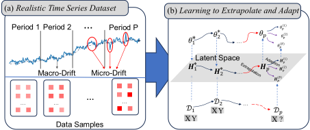
In this paper, we tackle the concept drift problem in online time series forecasting by addressing both macro-drifts and micro-drifts through a unified meta-learning framework named LEAF (Learning to Extrapolate and Adjust for Forecasting). Designed to be model-agnostic, LEAF is compatible with a variety of deep prediction models including MLPs, RNNs, CNNs, and Transformer-based models. By learning a lowdimensional latent embedding of the model parameters, LEAF adeptly navigates the model dynamics in response to concept drift, optimizing in a reduced space to both capture drift characteristics and mitigate over-fitting. The framework is articulated in two stages: an extrapolation stage to address stable, long-termmacro-drifts by learning and predicting their evolving patterns, and an adjustment stage that responds to unpredictable, short-term micro-drifts by adjusting model parameters with a sample-specific surrogate loss. Note that macro-drift typically corresponds to the long-term dynamics of time series, e.g., the dynamics of the trend or the seasonal component. Unlike the naive seasonal-trend decomposition which models these components directly, in the extrapolation stage we model it by learning a more powerful and adaptive meta-learned extrapolation network. This approach not only helps to capture evolving trends and dynamics but also enables real-time adjustment to abrupt changes, offering a comprehensive solution to handling concept drift in online forecasting scenarios. Our theoretical analysis, supported by empirical evidence from real-world applications, underscores the effectiveness of LEAF in improving forecasting accuracy in the presence of concept drift. We test the LEAF framework on various benchmark datasets extensively. It is incorporated into different deep learning algorithms including MLP, RNN, CNN and Transfornmer-based models. The experimental results verify its universal effectiveness and robustness across various scenarios and different forecasting algorithms 1 .
2 RelatedWork
Following the early success of LSTMmethods [Sutskever et al.2014, Salinas et al.2020] and CNN-based methods (e.g., TCN [Bai et al.2018]), Transformer-based models have surged to the forefront [Wen et al.2023] in forecasting, including LogTrans [Li et al.2019], Reformer [Kitaev et al.2020], Informer [Zhou et al.2021], Autoformer [Wu et al.2021], FEDformer [Zhou et al.2022], Quatformer [Chen et al.2022], etc. Some recent developments with SOTA performance include DLinear [Zeng et al.2023], PatchTST [Nie et al.2023], and TimesNet [Wu et al.2022]. Unfortunately, all these deep learning algorithms cannot handle concept drift quite well.
A common approach to address concept drift involves optimization-based meta-learning or model-based metalearning [Huisman et al.2021]. For example, DeepTime [Woo et al.2022] treats different lookback windows and forecast horizons as tasks, learning mappings from time indices to values that generalize effectively. [You et al.2021] treats historical and future data as tasks and utilizes Model-Agnostic MetaLearning (MAML) [Finn et al.2017] to adapt the model's parameters. Techniques initially developed for sequential domain adaptation and generalization, such as DDG-DA [Li et al.2022] and TDG [Liu et al.2023a], are also applicable to online time series forecasting, where they adapt the model to changing data distributions in various ways. In addition to meta-learning approaches, self-adaptive methods [Arik et al.2022] employ backcasting self-supervised objectives to enhance a model's adaptability to future distributions during prediction. FSNet [Pham et al.2023] introduces per-layer adapters and associative memory to dynamically adjust layer outputs and facilitate the learning of evolving patterns. SOLID [Chen et al.2024] proposes a detection and adaptation framework, which first quantifies model's susceptibility to the distribution shift, and then adapts the model with historical data sharing similar contexts on the sample-level. RevIN [Nie et al.2023] is a simple yet effective model-agnostic approach, which normalizes input samples before modeling and then reverses the process after making predictions. While these techniques collectively offer rich strategies to mitigate the challenges posed by concept drift, they fall short in adequately considering the specialties of concept drift in time series data.
1 Code, data and supplementary of the paper are available at https: //github.com/vc12301/LEAF
3 Methodologies
3.1 ProblemDefinition: Online Time Series Forecasting via Meta-Learning
Time series forecasting. A time series is an ordered sequence of observations denoted as Z = (z1, z2, · · · , zT ) ∈ RT×c , where T is the total number of time steps, zi ∈ Rc , and c is dimensionality. Time series forecasting aims at learning a prediction model fθ to predict the next O-steps at time t given a look-back window of length I as zt-I+1:t f (·;θ) ---→ zt+1:t+O, where θ is the model parameter. For simplicity, in the remainder of the paper, we denote the input zt-I+1:t and the output zt+1:t+O as x and y and a set of input and output as X and Y, respectively.
Online time series forecasting. Time series data often arrives in a streaming fashion with frequent concept drift. An appropriate approach is to continuously update the model over a sequence of periods. At each online forecasting period p, the model accesses and learns from the most recent data available and makes predictions for the future. Subsequently, the ground truth is revealed, allowing for updating the model once again. This cyclic process ensures that the model remains up-to-date and adapts to the changing nature of the time series.
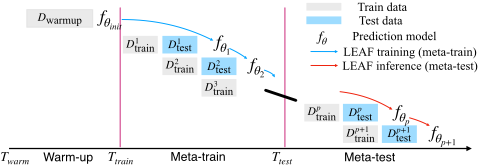
Meta-learning. Note that simply fitting a prediction model to the most recent observed data is insufficient due to concept drift, and the model needs to effectively generalize to future data. Meta-learning, also known as learning to learn, is a machine learning approach where a model learns how to learn from experience or previous tasks, enabling it to quickly adapt and generalize to new tasks. In the context of online time series forecasting, our objective is to learn how to adapt to future data. Our meta-learning based LEAF algorithm is trained over a sequence of online forecasting periods, referred as the meta-training phase, and evaluated over another sequence of periods called the meta-test phase. The procedure is depicted in Figure 2.
3.2 Learning to Extrapolate and Adjust
Model Overview. Formally, at each online forecasting period p, we have a training set Dp train = {Xp,Yp} and a test set Dp test = { ˜Xp, ˜Yp}. Without loss of generality, we assume that both the training set and the test set contain B samples. Specifically, Xp = {x(i) p }Bi=1 and ˜Xp = {˜x(i) p }Bi=1 . The main objective of LEAF is to leverage knowledge gained from historical periods and generate model parameters to make accurate forecasts on Dp test in the presence of concept drift. To achieve this goal, LEAF learns two functions: extrapolation E(·; ϕe) and adjustment A(·; ϕa), addressing macro- and micro-drift, respectively, to generate model parameters θp at period p. The objective can be formulated as:
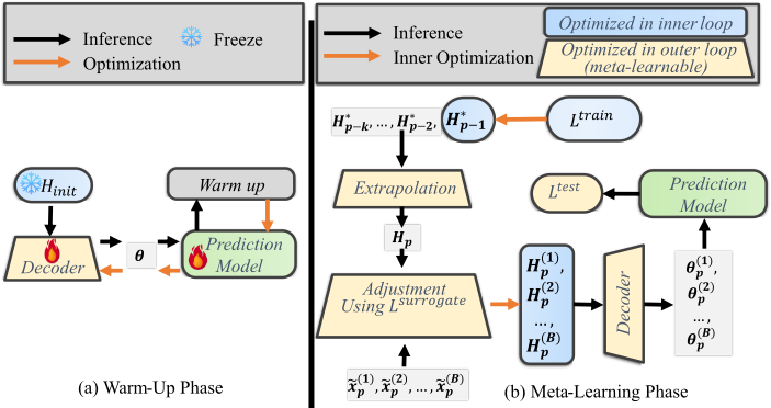
where the extrapolation function E(·;ϕe) is used to anticipate the macro-drift which takes as the optimal parameters θ∗p-k:p-1 from the previous k periods as input and infer parameters θp for period p, the adjustment function performs sample-specific parameter adjustment considering micro-drift within each sample, and L(·) is the prediction loss. Figure 3(b) illustrates the framework of LEAF.
Learning to Extrapolate in Latent Space
During the extrapolation stage, the meta-model LEAF aims at inferring a prediction model based on previously optimal models. To handle the possible concept drift especially macrodrift, we need to update the model effectively. In practice, we observe that often only a subset of patterns change in the concept while the majority remain invariant. In other words, we do not need to update all model parameters. To elegantly model it, we introduce a latent embedding H, which can be decoded to the model parameter θ, and the extrapolation is performed on this latent space.
In period p, we have Dp train = {Xp,Yp} and Dp test = { ˜Xp, ˜Yp}. In particular, Dp train is identical to the test data Dp-1 test , as shown in Figure 2. In other words, if we optimize the prediction model on Dp train , we can obtain the optimal model at period p - 1 in the latent space as follows:
where SGD represents gradient descent on Dp train with respect to prediction loss. This optimization process leads to the optimal latent embeddingH∗p-1 . Subsequently, we introduce an extrapolation network NN(·) that infers Hp based on the previous k optimal latent embeddings H∗p-k:p-1 and a decoder to generate model parameters, which can be formulated as:
Moving forward period p + 1, Dp test (or Dp+1 train ) is revealed. The above steps can be repeated to obtain H∗p , Hp+1 and θp+1. NN(·) can be any sequential model, e.g., LSTM and Transformer. We utilize a simple LSTM here as default to verify the capability of the framework itself. Besides, we investigate the network selection of the extrapolation network (see Supplementary A.6).
Learning to Adjust via Surrogate Loss
As the historical and forecast horizon of time series tend to coexist within an identical domain, it is quite beneficial to performmodel adaptation to capture the micro-drift at inference (test) time according to the input ˜X. To this end, we introduce a meta-learnable surrogate loss that adjusts or modulates the latent embedding Hp for each sample {˜x(i) p }Bi=1 in Dp test to obtain sample-specific embeddings {H(i) p }Bi=1 . This surrogate loss is implemented using neural networks and applied during the test phase, enabling the adjustment of the latent embedding based on sample-specific characteristics.
The rationale behind this approach is that micro-drift is often caused by external events, such as weather conditions or holidays. Although data affected by micro-drift may exhibit different patterns, they tend to deviate from their context in a similar manner. For example, the electricity consumption pattern during the summer typically differs from that in the winter, while during holidays it tends to decrease regardless of the season. By incorporating a meta-learnable surrogate loss, we aim to capture and adjust for these sample-specific deviations caused by micro-drift. Specifically, during the meta-training phase, the surrogate loss is learned to capture and compensate for different types of deviations. During the meta-testing phase, the model utilizes the learned surrogate loss to adjust the latent embedding based on the specific characteristics of each individual sample. To achieve this, the loss network takes into account the following three factors to capture samplespecific micro-drift: 1) Sample and base prediction.The sample itself ˜x(i) p and the base prediction with inferred model parameters in extrapolation stage f(˜x(i) p ; θp) are introduced as basic characteristics; 2) Base latent embedding. As we optimize the model in a latent space, the inferred latent embedding in the extrapolation stage Hp is passed to the loss network, providing the contextual information and underlying pattern; 3) Sample's relationship to training data. Furthermore, we introduce a relation network to account for sample's relationship to its context. The relation network R(·) receives embeddings of the sample ˜x(i) p and training set Dp train and returns a vector representing their relationship:
where g(·) is an embedding function, and the training data embedding is computed as the mean pooling of embeddings of all samples in the training set. The relation network captures the similarities or dissimilarities in their patterns, which is valuable in capturing the micro-drift. To sum up, the final loss network s(·) are defined as
The surrogate loss guides the adjustment of the latent embedding for each sample using gradient descent, which can be further decoded to obtain sample-specific model parameters:
where α is the learning rate, and H(i) p and θ(i) p stand for sample-specific latent embedding and model parameters, respectively. Finally, the parameters are loaded to make forecasts with f(˜x(i) p ); θ(i) p ).
Model Learning
In this subsection, we outline the training procedure of LEAF, as depicted in Algorithm 1. We denote the parameters of extrapolation module and adjustment module as ϕe and ϕa, respectively. Additionally, ω represents the parameter of the decoder.
At each period p, as shown in Figure 3(b), after extrapolation and adjustment stages (the "inner loop"), we make predictions on Dp test. The test set is then utilized to update the parameters of meta-learners ϕa, ϕe, ω (the "outer loop"). More precisely, the optimization process of "outer loop" is performed by minimizing the following objective:
where the first term is the prediction loss on the test set, the second term regularizes the extrapolation in Eq. (3) to output
Algorithm 1: Training Procedure of LEAF
Input: Number of meta-training periods P , data {Dp train , Dp test }Pp=1 , learning rates η, α, µ, number of historical periods in extrapolation stage k, prediction model f(·) 1 Randomly initialize the parameters ϕe , ϕa , and ω of LEAF ; 2 Let ψ = {ϕe ,ϕa ,ω} ; 3 Randomly initialize the latent embeddingH0 ; 4 Create a queue Q of size k storing the recent k optimal latent embeddings; 5 Initialize Q as Q = [H0, · · · ,H0] ; 6 for p = 1, 2, · · · , P do 7 Evaluate inner-loop prediction loss Ltrain p on training dataset Dp train ; 8 Perform gradient descent H∗p-1 = Hp-1 - η∇Hp-1 Ltrain p ; 9 Q.Deque().Enque(H∗p-1 .detach()) 10 ComputeHp and θp using Eq. (3); /* Extrapolation stage */ 11 for ˜x(i) p in ˜Xp do 12 /* Adjustment stage: traverse all test inputs, and conduct sample-specific adjustment */ 13 Compute Lsurrogate (˜x(i) p ) using Eq. (5); 14 H(i) p =Hp -α∇Hp Lsurrogate (˜x(i) p ); 15 θ(i) p = Decoder(H(i) p ), and load θ(i) p into f(·); 16 Evaluate prediction loss Ltest p,i w.r.t. ˜x(i) p ; 17 end 18 Compute LLEAF using Eq. (7); 19 Perform gradient descent ψ = ψ - µ∇ψLLEAF ; 20 endlatent embedding that is close to the optimal latent embedding, and γ is the coefficient of the regularization.
Recall that online forecasting often involves a warm-up phase. Since we optimize the parameters of the prediction model in the latent space, the traditional training strategy is not directly applicable. To address this issue, we randomly generate a latent embedding Hinit, which is then decoded into parameters of prediction model using the decoder. During the training procedure of the warm-up phase, Hinit remains fixed and the decoder is trained using the prediction loss on warmup dataset. Subsequently, at the onset of the meta-learning, we initialize H0 with Hinit and ω with the learned decoder parameter from warm-up phase. Figure 3(a) illustrates the warm-up strategy.
Remarks. LEAF generates the parameters for the last few layers of the target prediction model. It is important to note that LEAF is a model-agnostic framework, allowing different types of layers. For instance, when using DLinear as the target prediction model, we could generate the parameters for the linear layer. In the case of PatchTST, we could generate the parameters for the last transformer block, which includes the Query/Key/Value projection networks and a feedforward network. To apply LEAF to different types of layers, we require the parameter shapes of the network layers. By flattening the parameters to be generated, we can determine the width of the decoder in LEAF. The generated parameters are then appropriately reshaped and loaded into the respective layers, allowing for flexibility and compatibility across different network architectures.
3.3 Theoretical Analysis
In this section, we provide a theoretical analysis for the simplified scenarios to justify our LEAF framework, where we assume a linear model ˆy =Wx for the forecasting task. During each online forecasting period p, the dataset {Xp,Yp}
is drawn from Pp, and we define that feature-target pair z = [x; y]. Assuming that we need to forecast at the current period P + 1, with optimal parameters obtained from the preceding periods, and our objective is to learn weights WP+1 that generalizes well at period P +1. In the simplified analysis, we introduce two mild conditions to characterize maco-drift and micro-drift.
Assumption 1 (Macro-drift). Pp+1, the data distribution for period P + 1, is a composite of Pp and an unknown distribution P∆ that accounts for macro-drift and is independent of Pp.
Assumption 2 (Micro-drift). A transformed sample z′ = f (z, P)+ϵ embodies micro-drift, and f (z, P) = z+αΣ- 12 (z-µ) is a deterministic function with unknown scalar α responsible for the incremental change within each sample considering its distribution context; µ and Σ stand for mean and covariance of P; ϵ follows a normal distribution N(0, diag(σ2 )) denoting the stochastic noise. We denote this data distribution as P ′ .
We summarize the theoretical analysis results by the following two propositions, with proofs provided in the Supplementary A.1.
Proposition 1. Given the complete datasets from preceding periods {Xp,Yp}Pp=1 , the associated optimal weights {W∗ p }Pp=1 and the input data {XP+1} for period P + 1. We approximate weights for period P + 1 as
This estimation exhibits much more generalization than the estimation with the last period:
Proposition 2. Considering the micro-drift, We possess the dataset {X′p,Y′p}Pp=1 , the associated optimal weights {W∗ p }Pp=1 and the input data {X′P+1} for period P + 1. A sample-level weight adjustment achieves less prediction error than weight estimation in Proposition 1:
Proposition 2 states that introducing a sample-dependent weight modification can alleviate the micro-drift. It implies that performing the sample-specific weight adjustment can reduce the prediction error in the context of sample-level microdrift.
Although our theoretical framework focuses on simplified linear models, the insights are highly relevant to real-world applications. This relevance is underscored by the fact that in numerous practical scenarios, only the parameters in the final linear layer of deep neural networks are updated, aligning with our theoretical approach. Moreover, even for nonlinear layers, practical evidence supports the effectiveness of our extrapolation and adjustment principles, which is supported in Table 3 in Supplementary where LEAF is applied to the last linear layer of a complex deep model.
| Model | Method | Load-1 | Load-2 | Load-3 | ETTh2 | ETTm1 | ECL | ||||||
|---|---|---|---|---|---|---|---|---|---|---|---|---|---|
| MSE | MAE | MSE | MAE | MSE | MAE | MSE | MAE | MSE | MAE | MSE | MAE | ||
| Na¨ıve | 2.0153 | 1.0274 | 1.8738 | 0.9860 | 3.9113 | 1.3920 | 0.8091 | 0.6315 | 2.2219 | 0.9526 | 0.1805 | 0.2726 | |
| Na¨ıve† | 1.5716 | 0.8683 | 1.6839 | 0.9082 | 2.8948 | 1.1320 | 0.9067 | 0.6432 | 1.3905 | 0.7421 | 0.1527 | 0.2494 | |
| Retrain | 1.4062 | 0.8158 | 1.5189 | 0.8562 | 2.7411 | 1.0829 | 0.8796 | 0.6367 | 1.2866 | 0.7109 | 0.1480 | 0.2449 | |
| LSTM | Fine-tune | 1.4352 | 0.8214 | 1.5186 | 0.8523 | 3.0643 | 1.1393 | 0.7684 | 0.6096 | 1.4441 | 0.7449 | 0.1546 | 0.2459 |
| ER | 1.4358 | 0.8215 | 1.5081 | 0.8482 | 3.0211 | 1.1323 | 0.7662 | 0.6072 | 1.4106 | 0.7352 | 0.1511 | 0.2441 | |
| DER++ | 1.4338 | 0.8215 | 1.5012 | 0.8454 | 2.9956 | 1.1297 | 0.7541 | 0.6042 | 1.3953 | 0.7311 | 0.1509 | 0.2443 | |
| SOLID* | 1.3790 | 0.7935 | 1.5009 | 0.8480 | 2.7509 | 1.0718 | 0.7574 | 0.6018 | 1.4257 | 0.7396 | 0.1461 | 0.2408 | |
| LEAF | 0.6111 | 0.4728 | 0.6414 | 0.5057 | 1.7328 | 0.7993 | 0.7202 | 0.5874 | 0.7392 | 0.5447 | 0.1264 | 0.2187 | |
| Na¨ıve | 0.6664 | 0.4974 | 0.6507 | 0.4855 | 1.9434 | 0.8767 | 0.6790 | 0.5597 | 0.7506 | 0.5410 | 0.1277 | 0.2134 | |
| Na¨ıve† | 0.6381 | 0.4805 | 0.6287 | 0.4766 | 1.8153 | 0.8191 | 0.7531 | 0.5738 | 0.6615 | 0.4982 | 0.1228 | 0.2075 | |
| Retrain | 0.6240 | 0.4738 | 0.6098 | 0.4735 | 1.8067 | 0.8121 | 0.7448 | 0.5722 | 0.6652 | 0.4990 | 0.1224 | 0.2072 | |
| DLinear | Fine-tune | 0.7231 | 0.5210 | 0.6809 | 0.5095 | 2.1164 | 0.9080 | 0.6461 | 0.5491 | 0.7226 | 0.5220 | 0.1261 | 0.2106 |
| ER | 0.7135 | 0.5152 | 0.6756 | 0.5059 | 2.0879 | 0.8992 | 0.6603 | 0.5511 | 0.7083 | 0.5165 | 0.1248 | 0.2093 | |
| DER++ | 0.7053 | 0.5100 | 0.5026 | 2.0617 | 0.8907 | 0.6567 | 0.5495 | 0.6990 | 0.5131 | 0.1244 | 0.2093 | ||
| SOLID* | 0.5046 | 0.6709 | 0.5004 | 1.9939 | 0.8700 | 0.6453 | 0.5482 | 0.7048 | 0.5078 | ||||
| 0.6792 | 0.6711 | 0.1249 | 0.2092 | ||||||||||
| LEAF | 0.6039 | 0.4602 | 0.5866 | 0.4564 | 1.7172 | 0.7773 | 0.6450 | 0.5487 | 0.6128 | 0.4818 | 0.1144 | 0.2055 | |
| Na¨ıve | 2.2288 | 1.0823 | 0.9735 | 0.6846 | 2.5516 | 1.0626 | 0.8103 | 0.6225 | 1.5935 | 0.7805 | 0.1429 | 0.2274 | |
| Na¨ıve† | 0.7442 | 0.5700 | 0.6716 | 0.5250 | 1.8921 | 0.8887 | 0.7247 | 0.5813 | 0.6426 | 0.5089 | 0.1140 0.1130 | 0.2081 | |
| PatchTST | Retrain Fine-tune | 0.6614 0.9613 | 0.5262 0.6424 | 0.6233 0.8540 | 0.5074 0.6193 | 1.7995 2.7340 | 0.8471 1.0980 | 0.7206 0.6894 | 0.5789 0.5736 | 0.6412 0.8871 | 0.5032 0.5940 | 0.1238 | 0.2069 0.2142 |
| ER | 0.8658 | 0.6154 | 0.7813 | 0.5891 | 2.3152 | 0.9931 | 0.6901 | 0.5716 | 0.8088 | 0.5631 | 0.1199 | 0.2114 | |
| DER++ | 0.8285 | 0.5972 | 0.7538 | 0.5731 | 2.2190 | 0.9625 | 0.6824 | 0.5677 | 0.7712 | 0.5479 | 0.1193 | 0.2104 | |
| SOLID* | 0.8733 | 0.6188 | 0.7536 | 0.5801 | 2.3169 | 0.9946 | 0.6878 | 0.5706 | 0.7473 | 0.5435 | 0.1161 | 0.2095 | |
| LEAF | 0.6466 | 0.6233 | 0.5072 | 1.9230 | 0.2046 | ||||||||
| 0.5132 | 0.8787 | 0.6746 | 0.5654 | 0.6673 | 0.5070 | 0.1154 | |||||||
| Na¨ıve | 1.1432 | 0.7265 | 1.2994 | 0.8000 | 3.2940 | 1.2296 | 0.8959 | 0.6784 | 1.8551 | 0.8710 | 0.1541 | 0.2676 | |
| Na¨ıve† | 0.9074 | 0.6417 | 1.0625 | 0.6972 | 2.6903 | 1.0952 | 0.8996 | 0.6648 | 1.2383 | 0.7156 | 0.1390 | 0.2534 | |
| Retrain | 0.8590 | 0.6176 | 1.0154 | 0.6898 | 2.7245 | 1.0872 | 0.8790 | 0.6605 | 1.3906 | 0.7427 | 0.1368 | 0.2503 | |
| TCN | Fine-tune | 0.9880 | 0.6590 | 1.1706 1.1591 | 0.7359 | 3.0837 2.9623 | 1.1796 1.1467 | 0.8148 | 0.6391 | 1.4536 | 0.7633 0.7238 | 0.1387 0.1413 | 0.2523 |
| ER DER++ | 0.9416 0.9417 | 0.6381 | 1.1357 | 0.7295 0.7160 | 2.9769 | 1.1511 | 0.8189 0.8099 | 0.6400 0.6381 | 1.3063 1.2877 | 0.7141 | 0.1366 | 0.2529 0.2504 | |
| FSNet | 0.8114 | 0.6337 | 0.5524 | 2.2620 | 0.8277 | 0.9732 | 0.6370 | 0.1655 | 0.2778 | ||||
| 0.5607 | 0.7315 | 0.9506 | 1.4667 | ||||||||||
| SOLID* | 0.9589 | 0.6395 | 0.9836 | 0.6806 | 2.8407 | 1.1169 | 0.7643 | 0.6153 | 1.2735 | 0.7058 | 0.1333 | 0.2509 | |
| LEAF | 0.6834 | 0.5222 | 0.6539 | 1.8516 | 0.5827 | 0.9201 | 0.5976 | 0.1171 | 0.2327 | ||||
| Na¨ıve | 1.2964 | 0.7812 | 0.9809 | 0.5200 0.6851 | 2.3778 | 0.8474 1.0097 | 0.7093 0.9144 | 0.6737 | 1.8664 | 0.8842 | 0.2125 | 0.2962 | |
| Na¨ıve† Retrain | 1.2444 1.1212 | 0.7687 0.7375 | 0.9790 0.9849 | 0.6854 0.6911 | 2.3823 2.2698 | 1.0276 0.9986 | 0.8817 0.8677 | 0.6536 0.6510 | 1.3899 1.3588 | 0.7641 0.7469 | 0.1794 0.1719 | 0.2702 | |
| TimesNet | Fine-tune | 1.1328 | 0.7352 | 0.9965 | 0.6951 | 2.3408 | 1.0173 | 0.7952 | 0.6298 | 1.4097 | 0.7638 | 0.1656 | 0.2646 0.2864 |
| ER | 2.3589 | 1.0131 | 0.2549 | ||||||||||
| DER++ | 1.1054 | 0.7347 | 0.9832 | 0.6905 | 2.3132 | 0.8137 | 0.6369 | 1.3645 | 0.7526 | 0.1636 | 0.2568 | ||
| SOLID* | 1.1816 | 0.7571 | 0.9677 | 0.6858 | 1.0037 | 0.7981 | 0.6318 0.6092 | 1.3786 1.2052 | 0.7542 0.7087 | 0.1655 | |||
| LEAF | 1.1053 | 0.7282 | 0.9418 | 0.6805 | 2.2778 | 1.0034 | 0.7384 | 0.1607 | 0.2504 | ||||
| 0.6601 | 0.5029 | 0.6328 | 0.5053 | 1.7931 | 0.8247 | 0.6939 | 0.5806 | 0.7668 | 0.5486 | 0.1226 | 0.2186 | ||
4 Experiments
In this section, we conduct experiments to answer two questions: (RQ1) Can LEAF outperform SOTA model-agnostic concept drift adaptation methods in online time series forecasting scenarios? (RQ2) How do different components of LEAF contribute to resolving concept drift problems?
4.1 Experimental Settings
Datasets. We evaluate our method on six time series forecasting datasets. (1) ETT-small 2 [Zhou et al.2021] dataset contains observations of oil temperature along with six power load features over two years. For ETTh2, the model update interval (number of timesteps in each Dtrain) is 288, the lookback window is 96 and the forecast horizon is 24. For ETTm1, the model update interval is 672, the look-back window is 288 and the forecast horizon is 24. (2) ECL 3 dataset records hourly electricity consumption of 321 users over three years. We randomly sample 12 users. The model update interval is 288, the look-back window is 96 and the forecast horizon is 24. (3) Load dataset contains three real-world univariate electric load benchmarks in different types of areas at 15-minute intervals from 2020 to 2022. Figure 4 and Figure 5 ( in Supplementary A.2) visually demonstrate the presence of concept drift within each benchmark, including various types of macro and micro drifts. More details of the dataset are included in Supplementary A.2. Results with different forecast horizons
2 https://github.com/zhouhaoyi/ETDataset
3 https://archive.ics.uci.edu/dataset/321/ electricityloaddiagrams20112014
(ranging from 48 to 336) are shown in Table 5. Results on more datasets (NASDAQ-100 and WTH from economic and meteorological domains, respectively) are included in Supplementary A.3 and case studies on the forecast abilies of LEAF under concept drift are included in Supplementary A.8.
Baselines. We compare our method with multiple modelagnostic baselines, including: (1) Na¨ıve: it only warms-up the model and then freezes henceforth; (2) Na¨ıve†: it trains on warm-up and meta-train dataset and then freezes at meta-test; (3) Retrain: it updates the last few layers of backbone model at each period by gradient descent using all available data; (4) Fine-tune: it updates the last few layers of backbone model at each period by gradient descent using only the data in the period; (5) ER [Chaudhry et al.2019]: it employs a memory bank of most recent samples; (6) DER++ [Buzzega et al.2020]: a variate of ER with knowledge distillation; and (7) SOLID [Chen et al.2024]: a detection and adaptation framework that first quantifies model's susceptibility to distribution shift and then adapts the model with historical data sharing similar contexts on the sample-level. Since the original work employs an offline approach, we implement a variant SOLID* that continually fine-tunes the model parameters for fair comparison. We also compare our method with FSNet [Pham et al.2023], a recent SOTA for concept drift in online time series forecasting that uses TCN [Bai et al.2018] as the backbone and incorporates an experience replay. More details of baselines are included in Supplementary A.5.
Implementation Details. For all benchmarks, we split the data into warm-up/meta-train/meta-test by the ratio of 0.1/0.6/0.3. In warm-up phase, we use Adam [Kingma and Ba2014] with fixed learning rate of 0.001 to optimize the prediction model wrt the mean squared loss. The warm-up epoch is 10 and warm-up batch size is 32. In meta-training and meta-testing phases, at each period p, we use Adam with learning rate of 0.001 to obtain the optimal latent embedding and update parameters of meta-learners, the update epoch is 50 and 1, respectively. We implement Decoder, relation network R(·), and loss network s(·) with MLPs. We perform crossvalidation on meta-train to select appropriate hyper-parameters for all methods. We notice that LEAF is able to achieve competitive results with minor hyperparameter tuning. We report the hyperparameter sensitivity in Supplementary A.6. Besides, all baselines are well-tuned using Bayesian optimization from Neural Network Intelligence toolkit 4 . All experimental results are the average of the five independent trials with different random seeds.
4.2 Performance Comparison (RQ1)
The results of comparison performance are shown in Table 1 and the standard deviations are shown in Table 11. We apply model-agnostic methods to five types of prediction models, including LSTM [Hochreiter and Schmidhuber1997], DLinear [Zeng et al.2023], PatchTST [Nie et al.2023], TimesNet [Wu et al.2022] and TCN [Bai et al.2018]. We place FSNet [Pham et al.2023] in TCN category since it employs a TCN-based backbone. More details of backbone prediction models are included in Supplementary A.5. We use mean squared error (MSE) and mean absolute error (MAE) as evaluation metrics and they are averaged over meta-test periods. From Table 1, we can observe that: (1) our proposed LEAF significantly improves forecast performance in almost all cases, especially in Load benchmarks, for different types of prediction models. Overall, LEAF has a 14.4% reduction in error compared with second-best method. Especially, LEAF has an average decrease of 35.4% in MSE when using LSTM as prediction model, 29.5% when using TimesNet; (2) LEAF performs surprisingly well on Load-1, Load-2, and ETTm1 datasets, while the advantage is not so obvious on ECL dataset. This is because time series from Load-1, Load-2, and ETTm1 datasets exhibit much stronger and more complex concept drift; (3) Retrain, ER and DER++ show competitive performance in ECL dataset, as time series in this dataset holds strong seasonality and recurring patterns. These methods incorporate a memory of samples which helps alleviate catastrophic forgetting and remembering recurring patterns in history. We note here ER and its variant are orthogonal to our work which can be embedded easily into LEAF. Moreover, we report the running time complexity of different fine-tune methods in Tables 7, 8 and 9, wherein LEAF is not significantly more computationally expensive than Fine-tune, despite its superior performance compared to Fine-tune. Besides, sample-specific adjustment does not significantly contribute to the computational burden, as the adjustment is performed on latent space for one iteration. The complete running time comparison experiments are in Supplementary A.4.
4 https://nni.readthedocs.io/en/stable
| Model | Method | Load-1 | ETTm1 | ||
|---|---|---|---|---|---|
| MSE | MAE | MSE | MAE | ||
| DLinear | Fine-tune | 0.7231 | 0.5210 | 0.7226 | 0.5220 |
| Latent fine-tune | 0.6683 | 0.5057 | 0.7019 | 0.5196 | |
| Latent fine-tune + A | 0.6562 | 0.5045 | 0.6745 | 0.5295 | |
| EN | 0.6578 | 0.4931 | 0.6723 | 0.5066 | |
| EN + A | 0.6039 | 0.4602 | 0.6128 | 0.4818 | |
| PatchTST | Fine-tune | 0.9613 | 0.6424 | 0.8871 | 0.5940 |
| Latent fine-tune | 0.8103 | 0.6068 | 0.7546 | 0.5473 | |
| Latent fine-tune + A | 0.6783 | 0.5198 | 0.6823 | 0.5143 | |
| EN | 0.7539 | 0.5800 | 0.7334 | 0.5410 | |
| EN + A | 0.6466 | 0.5132 | 0.6673 | 0.5070 | |
4.3 Ablation Studies (RQ2)
We conduct ablation studies to validate the effectiveness of extrapolation and adjustment modules. We evaluate the performance of five variants of LEAF upon DLinear and PatchTST. Considering that LEAF can be treated as an advanced method of fine-tuning, we begin with the most basic fine-tuning method and gradually incorporate designed modules in LEAF to construct thevariants. The variants include: (1) Fine-tune that is foundation of LEAF and is performed in the parameter space; (2) Latent fine-tune performs fine-tuning in the latent space that uses an average of last five H∗ instead of the extrapolated latent embedding H; (3) EN that introduces the extrapolation module; (4) Latent fine-tune + A that incorporates the adjustment stage; and (5) EN + A that incorporates the adjustment stage on extrapolation module and is identical to standard LEAF.
The results are shown in Table 2. We observe first that fine-tuning model in the latent space (Latent fine-tune) can significantly improve the forecast performance in almost all benchmarks. This outcome verifies that optimizing model in a low-dimensional latent space is rational. Furthermore, EN introducing our proposed extrapolation module surpasses the performance of Latent fine-tune, thereby confirming its effectiveness in extrapolating the macro-drift. Lastly, the inclusion of the sample-specific adjustment yields a further enhancement in predictive performance, demonstrating the effectiveness of this stage in alleviating micro-drift. Moreover, we plot prediction results of different variants in Figure 7 (see Supplementary A.7).
5 Conclusion and FutureWork
In conclusion, our proposed LEAF framework offers a promising solution to the concept drift problem in online time series forecasting. By integrating meta-learning, LEAF enhances the capabilities of deep prediction models by acquiring the ability to extrapolate and adapt to macro- and micro-drift, respectively. This model-agnostic framework can be applied to various deep prediction models, making it versatile and applicable in different domains. In the future, we plan to extend our framework to handle more intricate concept drift scenarios, and one potential direction is the combination of LEAF and continual learning methods.
@inproceedings{ijcai2025p542,
  title     = {Learning to Extrapolate and Adjust: Two-Stage Meta-Learning for Concept Drift in Online Time Series Forecasting},
  author    = {Chen, Weiqi and Zhu, Zhaoyang and Zhang, Yifan and Shen, Lefei and Yang, Linxiao and Wen, Qingsong and Sun, Liang},
  booktitle = {Proceedings of the Thirty-Fourth International Joint Conference on
               Artificial Intelligence, {IJCAI-25}},
  publisher = {International Joint Conferences on Artificial Intelligence Organization},
  editor    = {James Kwok},
  pages     = {4869--4877},
  year      = {2025},
  month     = {8},
  note      = {Main Track},
  doi       = {10.24963/ijcai.2025/542},
  url       = {https://doi.org/10.24963/ijcai.2025/542},
}
TY - CPAPER TI - Learning to Extrapolate and Adjust: Two-Stage Meta-Learning for Concept Drift in Online Time Series Forecasting AU - Chen, Weiqi AU - Zhu, Zhaoyang AU - Zhang, Yifan AU - Shen, Lefei AU - Yang, Linxiao AU - Wen, Qingsong AU - Sun, Liang T2 - Proceedings of the Thirty-Fourth International Joint Conference on Artificial Intelligence, IJCAI-25 PB - International Joint Conferences on Artificial Intelligence Organization PY - 2025 SP - 4869 EP - 4877 DO - 10.24963/ijcai.2025/542 UR - https://doi.org/10.24963/ijcai.2025/542 ER -Copied
Machine-readable versions of this paper, for tools and AI agents:





