
Pseudo-Label Reconstruction for Partial Multi-Label Learning
Proceedings of the Thirty-Fourth International Joint Conference on Artificial Intelligence. Main Track. Pages 4896-4904.
https://doi.org/10.24963/ijcai.2025/545
Keywords
- Constraint Satisfaction and Optimization: CSO: Constraint optimization problems
- Machine Learning: ML: Regression
- Machine Learning: ML: Multi-label learning
- Machine Learning: ML: Optimization
Abstract
In Partial Multi-Label Learning (PML), each instance is associated with a candidate label set containing multiple relevant labels along with other false positive labels. Currently, most PML methods directly extract instance correlation from instance features while ignoring the candidate labels, which may contain more discriminative instance-related information. This paper argues that, with a well-designed model, more accurate instance correlation can be mined from the candidate labels to facilitate label disambiguation. To this end, we propose a novel PML method based on pseudo-label reconstruction (PML-PLR). Specifically, we first propose a novel orthogonal candidate label reconstruction method, which jointly optimizes with instance features to extract more consistent instance correlation. Then, we use instance correlation as reconstruction coefficient to reconstruct pseudo-labels. Subsequently, through local manifold learning, the reconstructed pseudo-labels are leveraged to propagate the consistency relationship between labels and instances, thereby improving the accuracy of pseudo-labels. Extensive experiments and analyses demonstrate that the proposed PML-PLR outperforms state-of-the-art methods.
- [Cai et al., 2010] Jian-Feng Cai, Emmanuel J Candès, and Zuowei Shen. A singular value thresholding algorithm for matrix completion. SIAM Journal on optimization, 20(4):1956-1982, 2010.
- [Chen et al., 2024] Yu Chen, Yanan Wu, Na Han, Xiaozhao Fang, Bingzhi Chen, and Jie Wen. Partial multi-label learning based on near-far neighborhood label enhance- ment and nonlinear guidance. In ACM Multimedia 2024, 2024.
- [Demšar, 2006] Janez Demšar. Statistical comparisons of classifiers over multiple data sets. The Journal of Machine learning research, 7:1-30, 2006.
- [Fang et al., 2025] Xiaozhao Fang, Xi Hu, Yan Hu, Yong- hao Chen, Shengli Xie, and Na Han. Fuzzy bifocal dis- ambiguation for partial multi-label learning. Neural Net- works, 185:107137, 2025.
- [Feng et al., 2020] Lei Feng, Jun Huang, Senlin Shu, and Bo An. Regularized matrix factorization for multilabel learning with missing labels. IEEE transactions on cy- bernetics, 52(5):3710-3721, 2020.
- [Han et al., 2025] Qingqi Han, Liang Hu, and Wanfu Gao. Integrating label confidence-based feature selec- tion for partial multi-label learning. Pattern Recognition, 161:111281, 2025.
- [Hang and Zhang, 2023] Jun-Yi Hang and Min-Ling Zhang. Partial multi-label learning with probabilistic graphical disambiguation. Advances in Neural Information Process- ing Systems, 36:1339-1351, 2023.
- [Hao et al., 2023] Pingting Hao, Liang Hu, and Wanfu Gao. Partial multi-label feature selection via subspace optimiza- tion. Information Sciences, 648:119556, 2023.
- [Hou et al., 2016] Peng Hou, Xin Geng, and Min-Ling Zhang. Multi-label manifold learning. In Proceedings of the AAAI conference on artificial intelligence, volume 30, 2016.
- [Hu et al., 2023] Yan Hu, Xiaozhao Fang, Peipei Kang, Yonghao Chen, Yuting Fang, and Shengli Xie. Dual noise elimination and dynamic label correlation guided partial multi-label learning. IEEE Transactions on Multimedia, 2023.
- [Huang et al., 2015] Jin Huang, Feiping Nie, Heng Huang, et al. A new simplex sparse learning model to measure data similarity for clustering. In IJCAI, pages 3569-3575, 2015. IJCAI
- [Li et al., 2021] Ziwei Li, Gengyu Lyu, and Songhe Feng. Partial multi-label learning via multi-subspace represen- tation. In Proceedings of the Twenty-Ninth International Conference on International Joint Conferences on Artifi- cial Intelligence, pages 2612-2618, 2021. IJCAI
- [Li et al., 2022] Feng Li, Shengfei Shi, and Hongzhi Wang. Partial multi-label learning via specific label disambigua- tion. Knowledge-Based Systems, 250:109093, 2022.
- [Lin et al., 2025] Yaojin Lin, Yulin Li, Shidong Lin, Lei Guo, and Yu Mao. Partial multi-label feature selection based on label distribution learning. Pattern Recognition, 164:111523, 2025.
- [Liu et al., 2021] Weiwei Liu, Haobo Wang, Xiaobo Shen, and Ivor W Tsang. The emerging trends of multi-label learning. IEEE transactions on pattern analysis and ma- chine intelligence, 44(11):7955-7974, 2021.
- [Liu et al., 2023] Bing-Qing Liu, Bin-Bin Jia, and Min-Ling Zhang. Towards enabling binary decomposition for partial multi-label learning. IEEE transactions on pattern analy- sis and machine intelligence, 2023.
- [Lyu et al., 2020] Gengyu Lyu, Songhe Feng, and Yidong Li. Partial multi-label learning via probabilistic graph matching mechanism. In Proceedings of the 26th ACM SIGKDD International Conference on Knowledge Discov- ery & Data Mining, pages 105-113, 2020.
- [Lyu et al., 2021] Gengyu Lyu, Songhe Feng, and Yidong Li. Noisy label tolerance: A new perspective of partial multi- label learning. Information Sciences, 543:454-466, 2021.
- [Mirone and Paleo, 2017] Alessandro Mirone and Pierre Pa- leo. A conjugate subgradient algorithm with adaptive pre- conditioning for the least absolute shrinkage and selection operator minimization. Computational Mathematics and Mathematical Physics, 57:739-748, 2017.
- [Qian et al., 2024a] Wenbin Qian, Yanqiang Tu, Jintao Huang, and Weiping Ding. Partial multi-label learning via robust feature selection and relevance fusion optimization. Knowledge-Based Systems, 286:111365, 2024.
- [Qian et al., 2024b] Wenbin Qian, Yanqiang Tu, Jintao Huang, Wenhao Shu, and Yiu-Ming Cheung. Partial mul- tilabel learning using noise-tolerant broad learning sys- tem with label enhancement and dimensionality reduction. IEEE Transactions on Neural Networks and Learning Sys- tems, 2024.
- [Sun et al., 2019] Lijuan Sun, Songhe Feng, Tao Wang, Con- gyan Lang, and Yi Jin. Partial multi-label learning by low-rank and sparse decomposition. In Proceedings of the AAAI conference on artificial intelligence, volume 33, pages 5016-5023, 2019.
- [Sun et al., 2021] Lijuan Sun, Songhe Feng, Jun Liu, Gengyu Lyu, and Congyan Lang. Global-local label corre- lation for partial multi-label learning. IEEE Transactions on Multimedia, 24:581-593, 2021.
- [Sun et al., 2024] Zhenzhen Sun, Zexiang Chen, Jinghua Liu, Yewang Chen, and Yuanlong Yu. Partial multi- label feature selection via low-rank and sparse factoriza- tion with manifold learning. Knowledge-Based Systems, 296:111899, 2024.
- [Tahzeeb and Hasan, 2022] Shahab Tahzeeb and S. M. Ma- mun Hasan. A neural network-based multi-label classifier for protein function prediction. Engineering, Technology & Applied Science Research, 2022.
- [Wang et al., 2019] Haobo Wang, Weiwei Liu, Yang Zhao, Chen Zhang, Tianlei Hu, and Gang Chen. Discrimina- tive and correlative partial multi-label learning. In IJCAI, pages 3691-3697, 2019. IJCAI
- [Wang et al., 2021] Qianqian Wang, Zhengming Ding, Zhiqiang Tao, Quanxue Gao, and Yun Fu. Generative partial multi-view clustering with adaptive fusion and cy- cle consistency. IEEE Transactions on Image Processing, 30:1771-1783, 2021.
- [Wang et al., 2022] Jing Wang, Peipei Li, and Kui Yu. Par- tial multi-label feature selection. In 2022 International Joint Conference on Neural Networks (IJCNN), pages 1-9. IEEE, 2022.
- [Wang et al., 2023] Qianqian Wang, Zhiqiang Tao, Wei Xia, Quanxue Gao, Xiaochun Cao, and Licheng Jiao. Adver- sarial multiview clustering networks with adaptive fusion. IEEE transactions on neural networks and learning sys- tems, 34:7635-7647, 2023.
- [Wang et al., 2024] Qianqian Wang, Zhiqiang Tao, Quanxue Gao, and Licheng Jiao. Multi-view subspace clustering via structured multi-pathway network. IEEE Transactions on Neural Networks and Learning Systems, 35(5):7244- 7250, 2024.
- [Wang et al., 2025] Ke Wang, Yahu Guan, Yunyu Xie, Zhao- hong Jia, Hong Ye, Zhangling Duan, and Dong Liang. Par- tial multi-label learning with label and classifier correla- tions. Information Sciences, 712:122101, 2025.
- [Wen et al., 2018] Jie Wen, Bob Zhang, Yong Xu, Jian Yang, and Na Han. Adaptive weighted nonnegative low-rank rep- resentation. Pattern Recognition, 81:326-340, 2018.
- [Wen et al., 2022] Jie Wen, Shijie Deng, Lunke Fei, Zheng Zhang, Bob Zhang, Zhao Zhang, and Yong Xu. Discrim- inative regression with adaptive graph diffusion. IEEE Transactions on Neural Networks and Learning Systems, 35(2):1797-1809, 2022.
- [Wen et al., 2023] Jie Wen, Gehui Xu, Zhanyan Tang, Wei Wang, Lunke Fei, and Yong Xu. Graph regularized and feature aware matrix factorization for robust incomplete multi-view clustering. IEEE Transactions on Circuits and Systems for Video Technology, 34(5):3728-3741, 2023.
- [Wu et al., 2025] You Wu, Peipei Li, and Yizhang Zou. Par- tial multi-label feature selection with feature noise. Pattern Recognition, 162:111310, 2025.
- [Xie and Huang, 2018] Ming-Kun Xie and Sheng-Jun Huang. Partial multi-label learning. In Proceedings of the AAAI conference on artificial intelligence, volume 32, 2018.
- [Xie and Huang, 2021] Ming-Kun Xie and Sheng-Jun Huang. Partial multi-label learning with noisy label identification. IEEE Transactions on Pattern Analysis and Machine Intelligence, 44(7):3676-3687, 2021.
- [Xie and Huang, 2022] Ming-Kun Xie and Sheng-Jun Huang. Ccmn: A general framework for learning with class-conditional multi-label noise. IEEE Transac- tions on Pattern Analysis and Machine Intelligence, 45(1):154-166, 2022.
- [Xu et al., 2020] Ning Xu, Yun-Peng Liu, and Xin Geng. Partial multi-label learning with label distribution. In Pro- ceedings of the AAAI conference on artificial intelligence, volume 34, pages 6510-6517, 2020.
- [Xu et al., 2023] Ning Xu, Yun-Peng Liu, Yan Zhang, and Xin Geng. Progressive enhancement of label distribu- tions for partial multilabel learning. IEEE transactions on neural networks and learning systems, 34(8):4856-4867, 2023.
- [Yu et al., 2018] Guoxian Yu, Xia Chen, Carlotta Domeni- coni, Jun Wang, Zhao Li, Zili Zhang, and Xindong Wu. Feature-induced partial multi-label learning. In 2018 IEEE international conference on data mining (ICDM), pages 1398-1403. IEEE, 2018.
- [Zhang and Fang, 2020] Min-Ling Zhang and Jun-Peng Fang. Partial multi-label learning via credible label elicita- tion. IEEE Transactions on Pattern Analysis and Machine Intelligence, 43(10):3587-3599, 2020.
- [Zhang and Wu, 2014] Min-Ling Zhang and Lei Wu. Lift: Multi-label learning with label-specific features. IEEE transactions on pattern analysis and machine intelligence, 37(1):107-120, 2014.
- [Zhang and Zhou, 2007] Min-Ling Zhang and Zhi-Hua Zhou. Ml-knn: A lazy learning approach to multi-label learning. Pattern recognition, 40(7):2038-2048, 2007.
- [Zhang and Zhou, 2013] Min-Ling Zhang and Zhi-Hua Zhou. A review on multi-label learning algorithms. IEEE transactions on knowledge and data engineering, 26(8):1819-1837, 2013.
- [Zhang et al., 2019] Jia Zhang, Zhiming Luo, Candong Li, Changen Zhou, and Shaozi Li. Manifold regularized dis- criminative feature selection for multi-label learning. Pat- tern Recognition, 95:136-150, 2019.
- [Zhang et al., 2024] Yao Zhang, Wei Huo, and Jun Tang. Multi-label feature selection via latent representation learning and dynamic graph constraints. Pattern Recog- nition, 151:110411, 2024.
- [Zhao et al., 2022a] Peng Zhao, Shiyi Zhao, Xuyang Zhao, Huiting Liu, and Xia Ji. Partial multi-label learning based on sparse asymmetric label correlations. Knowledge- Based Systems, 245:108601, 2022.
- [Zhao et al., 2022b] Tianna Zhao, Yuanjian Zhang, and Witold Pedrycz. Robust multi-label classification with en- hanced global and local label correlation. Mathematics, 10(11):1871, 2022.
- [Zhong et al., 2024] Jingyu Zhong, Ronghua Shang, Feng Zhao, Weitong Zhang, and Songhua Xu. Negative label and noise information guided disambiguation for partial multi-label learning. IEEE Transactions on Multimedia, 2024.
References were extracted automatically from the PDF and may contain errors.
Full text extracted automatically from the PDF; figures, tables and equations may differ. The PDF is the version of record.
1 Introduction
In the domain of machine learning, entities from the real world are often encapsulated as data points, each comprised of features and a corresponding label. In conventional classification tasks, labels are exclusive, allowing only a single label to be assigned to each data point. However, numerous real-world items possess multiple layers of meaning. Consider a film that might encompass genres like science fiction, war, and adventure, or a news piece that could be categorized under politics, economics, and sports. Multi-label learning (MLL) [Liu et al., 2021], which permits the assignment of multiple discrete labels to a single data point, has thus gained significant attention in machine learning circles and is utilized in a range of practical applications [Tahzeeb and Hasan, 2022], including: text classification, image recognition and protein function prediction. However, the process of acquiring datasets with accurate labels is not only costly but also difficult. More often, we may end up with just a candidate set of labels, some of which are relevant and others are just noise. This noise will blur the classification decision boundary, reducing the effectiveness of MLL.
∗Corresponding author
To address this challenge, Xie and Huang [Xie and Huang, 2018] propose the concept of partial multi-label learning (PML) as an innovative framework, whose objective is to build a model capable of assigning labels to new instances with noisy labels. The main challenge in PML is detecting noisy labels and building accurate classification models, which traditional multi-label learning (MLL) algorithms fail to address. For example, ML-KNN [Zhang and Zhou, 2007] and LIFT [Zhang and Wu, 2014] cannot effectively handle noisy labels, leading to poor performance on noisy datasets.
In recent years, the development of PML methods can be broadly categorized into two types: two-stage methods and end-to-end methods [Chen et al., 2024]. In two-stage methods, noisy labels are first identified and then the classifier is trained. Such as, DRAMA [Wang et al., 2019] constructs a label confidence matrix based on the feature manifold and candidate label set, utilizing it directly to train a multi-output regression model. PARTICLE [Zhang and Fang, 2020] applies label propagation to integrate information from K-nearest neighbors, establishes a confidence threshold for labels, and subsequently trains the MLC classifier. In contrast, end-toend methods optimize reliable labels and the classifier simultaneously. Examples include PML-DNDC [Hu et al., 2023] employs dual noise elimination, simultaneously removing label and feature noise to enhance classifier training by exploring label dependencies and promoting label similarity among classifiers. PML-ND [Zhong et al., 2024] employs negative label information to guide label propagation process to induce ground-truth labels with high credibility.
These methods address PML problems, but several critical limitations remain: 1) Existing approaches largely overlook the discriminative instance correlations embedded within candidate labels, primarily because noise contamination prevents direct extraction of meaningful correlations between instances. 2) Current disambiguation methods produce pseudolabels that inadequately capture the intrinsic consistency relationship between feature representations and label semantics, leading to suboptimal classification performance.
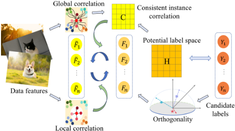
To address these limitations, this paper proposes a novel PML method based on pseudo-label reconstruction (PMLPLR). Specifically, we first introduce an innovative orthogonal candidate label reconstruction approach that leverages subspace reconstruction techniques to effectively mitigate both noise interference and complex label correlations within candidate label sets. This reconstruction is then jointly optimized with instance features to extract more robust and semantically meaningful instance correlations that better reflect true label relationships. Subsequently, these refined instance correlations serve as reconstruction coefficients to generate high-quality pseudo-labels that better approximate groundtruth labels. Finally, through local manifold learning, the reconstructed pseudo-labels propagate consistency relationships between features and labels, ensuring the final pseudolabels align more closely with the underlying true label distribution. The main framework is illustrated in Figure 1.
2 RelatedWork
2.1 Multi-Label Learning
In multi-label learning (MLL), each example is associated with multiple valid labels, and various approaches are extensively studied. Some methods transform MLL into binary classification problems, treating each label independently [Zhang et al., 2024]. To enhance performance, many studies explore label correlation, including pairwise and highorder dependencies. Recently, integrating manifold learning with MLL has gained increasing attention. Hou et al. [Hou et al., 2016] investigate the manifold structure in the label space, assuming that correlated instances share labels. Zhang et al. [Zhang et al., 2019] employ manifold learning and sparse feature selection to obtain a low-dimensional embedding for label information. Zhao et al. [Zhao et al., 2022b] combine manifold and subspace learning to mitigate noise and handle missing labels, reconstructing a more robust feature and label space. However, MLL typically assumes that each instance is precisely labeled, which is often unrealistic [Wang et al., 2024; Wang et al., 2023; Wang et al., 2021; Wen et al., 2023; Wen et al., 2022; Wen et al., 2018]. In noisy MLL, binary labels may be flipped to incorrect values. While these approaches reduce the burden of multi-label annotation, they neglect the inherent challenge of labeling-specifically, that labels themselves can be ambiguous.
2.2 Partial Multi-Label Learning
Compared to MLL, PML presents greater challenges, requiring learning in imperfect environments and training highprecision classifiers. Current PML research primarily centers on label disambiguation-identifying true labels within candidate sets. Existing approaches typically employ explicit learning strategies to remove noisy labels through various techniques. Some methods leverage low-rank and sparse decomposition to separate ground-truth labels from noise [Sun et al., 2019; Sun et al., 2024], while others estimate candidate label credibility via label propagation or enhancement techniques [Zhang and Fang, 2020; Xu et al., 2020; Xu et al., 2023; Lin et al., 2025; Chen et al., 2024]. Many approaches utilize feature information to identify noise [Yu et al., 2018; Xie and Huang, 2021; Wang et al., 2019; Lyu et al., 2021], with the most common practice being the application of correlation or manifold constraints on labels [Li et al., 2021; Lyu et al., 2020; Li et al., 2022; Hu et al., 2023]. Feature selection has recently emerged as a popular disambiguation strategy [Wang et al., 2022; Hao et al., 2023; Han et al., 2025; Wu et al., 2025], while other researchers harness label correlations or cluster assignments [Zhao et al., 2022a; Sun et al., 2021; Qian et al., 2024a; Wang et al., 2025; Fang et al., 2025]. Various deep learning algorithms have also been deployed to mine data distributions and mitigate noise impact [Hang and Zhang, 2023; Xie and Huang, 2022; Qian et al., 2024b].
3 ProposedMethod
In this section, we introduce PML-PLR and its feasibility optimization. Define some common variables as: X = [x1, x2, · · · , xn] ∈ Rd×n denotes feature matrix of n instances with d-dimensional features. Y ∈ {0, 1}l×n represents a candidate label matrix with noisy information, where l is the number of label classes. If Yij = 1 then the i-th label is associated with the j-th instance. If Yij = 0, the opposite. Each instance correspond to a set of candidate labels with unrelated labels incorrectly labeled as 1, which is called noisy label. The goal of PML is to minimize the impact of noisy information to make correct label predictions.
3.1 Learning Objective
Our ultimate goal is to induce a multi-label predictor f : X ↦→ [0, 1]l , which can assign an appropriate set of labels to unseen instances. The main objectives of this paper are as follows:
- Learning more consistent instance-level correlation, which allows the model to obtain more accurate correlation between instances.
- Learning label-instance relationships for pseudo-label reconstruction, which makes the generated pseudo-labels more consistent with instances and the real label distribution.
3.2 Instance-level Consistent Correlation Learning
The correlation between learning instances is typically measured using the feature similarity between each pair of instances. Common methods include the Gaussian kernel function, cosine similarity, and Pearson correlation coefficient. In order to learn instance-level correlation with higher consistency between features and labels, we first use the distance relationships of each instance's features to preliminarily learn the instance-level correlation. The formula is :
where, 1 is an n-dimensional all-1 row vector, C ∈ Rn×n represents the captured instance correlation matrix, each element cij reflects the influence of j-th instance on i-th instance. To enhance the consistency of instance-level correlation, we choose to use label information to jointly learn correlation. We believe that both features and labels are used to describe instances, and label information contains more discriminative instance correlation. We use label self-mapping to capture the correlation between instances without losing this discriminability. The formula is expressed as follows:
However, since label Y contains noise, C learned by the second item in the above method is not accurate enough. And due to the correlation between labels, some labels are highly related, leading to situations where two labels almost always appear together. To reduce the influence of label correlation and noise on instance-level correlation learning, for the second item, we select a more representative latent label space to learn more robust instance-level correlation. The formula is:
where H ∈ Rm×n (m ≤ l) represents the potential label space matrix, and P ∈ Rm×l is the indication matrix mapping the original label matrix to the latent label space. The constraint PP⊤ = Im ensures no distortion during dimensionality reduction, with the row vectors of P forming an orthogonal basis, meaning the column vectors of H are orthogonal components of Y in m-dimensional space. To mitigate information loss and dimensional sensitivity, we introduce a regularization term to preserve information flow. Specifically, we add a reconstruction term to retain key information from the original label matrix and a ℓ1-norm sparsity constraint to prevent overfitting due to noisy labels. The updated formula is as follows:
where α is a regularization parameter controlling the importance of preserving the original label structure. By updating Eq.(2), the learning formula of the final instance-level correlation is as follows:
3.3 Pseudo-label Reconstruction
In order to obtain better classification prediction results, pseudo-label learning should maintain high consistency between instances and labels while minimizing noise. Furthermore, to maximize the effectiveness of previously obtained instance-level correlation in subsequent pseudo-label reconstruction, we need to reduce the influence of incorrect instance correlations present in the original labels. We achieve this by utilizing a rotation transformation to alter the instance distribution, thereby weakening the instance correlations embedded in the original labels. This rotation-based approach is formulated as follows:
where F = [f1, f2, · · · , fn] ∈ Rl×n represents the pseudolabel matrix and Q ∈ Rn×n represents the orthogonal projection transformation matrix. By constraining Q to be orthogonal, the resulting pseudo-label matrix F preserves the essential structure while minimizing the misleading correlations inherited from the original label matrix Y. The constraint of 0l×n ≤ F ≤ Y can ensure that the main structure of the pseudo-label is consistent with the original label.
Next, we use the previously learned instance-level correlation C as the reconstruction coefficient to reconstruct the pseudo-labels, endowing them with the correct instance correlations. This approach follows the principle that similar instances should have similar labels. For the i-th instance fi, the instance-level correlation with other instances is used as label weight to reconstruct it. We can obtain reconstructed pseudo-label ˜fi:
To enhance the consistency between pseudo-labels and instances, we employ nearest neighbor relationships to constrain distances between pseudo-labels and their reconstructed counterparts. This approach ensures labels conform to the data's local manifold structure while propagating labelinstance relationships. The neighbor correlation is computed:
where N(xi) denotes the set of k nearest neighbors of sample xi, and σ = 1n ∑ni=1 ∥xi-x(k) i ∥2 is the bandwidth parameter of the Gaussian kernel, which controls how the distance between samples affects their similarity. The main goal of this section is to first weaken the instance-level correlation in the original labels using orthogonal mapping, then use the previously learned, more consistent instance-level correlation to reconstruct the pseudo-labels, and apply local manifold constraints to restore the instance-level correlation of the pseudolabels. The relationship between the label and the instance is propagated by reconstructing the pseudo-label. The overall formula for this section is expressed as follows:
3.4 Kernel Nonlinear Classifier
For the classifier part, we represent ϕ(·) : Rd → Rh as a feature mapping from the feature space to some h-dimensional high-dimensional Hilbert space, and then we can train the ridge regression model. Further using the deviation term b ∈ Rc in the prediction function, the prediction function with kernel extension can be expressed as g(xi) = W⊤ϕ(xi)+b. Supervised training using the pseudo-label F, then the classification model can be expressed as:
By defining a matrix E = [ϵ1, ϵ2, . . . , ϵ3]⊤∈ Rl×n the above problem can be re-written in the following matrix form:
where Φ = [ϕ(x1), ϕ(x2), . . . , ϕ(xn)]∈ Rh×n . To facilitate optimization, we restate Eq.(11) as:
3.5 Overall Objective Function
By combining the Eq.(5) (consistent correlation learning), Eq.(9) (pseudo-label learning and reconstruction) and Eq.(12) (classifier), the final objective function of the model is obtained as follows:
3.6 Optimization
For the above optimization problem, ADMM [Feng et al., 2020] is adopted to solve it. In other words, we use alternate optimization to solve Eq.(13), details are as follows:
Update P and H
Removing the items that are irrelevant to P and H, and fix C. Then, the sub-optimization as:
Then we apply the augmented Lagrange multiplier method to get the following Lagrange function:
where µ is a very large number. With P and E fixed, since PP⊤ = Im, H can be solved in a closed form :
With H and E fixed, for P, the sub-optimization can be converted to:
where Tr(·) is the trace norm. It is noted that the problem in Eq.(17) corresponds to the classic orthogonal procrustes problem [Cai et al., 2010], which can be approximated by singular value decomposition (SVD). Let R = 2YC⊤H⊤ + u(Y-E)H⊤, then we utilize SVD to decompose R, i.e., R = UΣV⊤, optimization of P can be obtained by:
With H and P fixed, the variables E can be optimized by solving following problem:
which is a typical LASSO regression problem [Mirone and Paleo, 2017], and we apply PGD algorithm to optimize it. The proximal operator of Eq.(19) is:
where Z = Et - 1L ∇L(E(t) ), E(t) represents the solution from the t-th iteration, and ∇L(E) is the gradient of the objective function L(E), L is the Lipschitz constant of ∇L(E) and t denotes the number of iteration. Problem of Eq.(20) can be iteratively updated by the soft-thresholding operator:
where Soft[b, ν] = sign(b)max{|b| -ν, 0}. In addition, the Lipschitz constant of ∇L(E) is 1, so we set L = 1.
Update C
Removing the items that are irrelevant toC, the suboptimization for C is simplified as:
where Lk is the Laplacian matrix of K, G ∈ Rn×n represents the distance matrix, for each element Gij = ∥xi -xj∥22 . Taking the derivative of Eq.(22) and setting the derivative to zero, we obtain the following equation:
Then, we can obtain the optimization result variable for the first step of optimizing C :
Then the optimization of C can be transformed into:
Eq (25) can be solved using the technique reported in [Huang et al., 2015] or be solved via off-the-shelf QP tools.
Update Q
For Q optimization, which also is a classical orthogonal problem, Q can be solved as: first compute the singular-value decomposition (SVD) of matrix Y⊤F as Y⊤F = MΣN⊤ and then let Q = MN⊤.
Update W and b
We add a bias term b to the classifier, so that classifier W becomes: Wm = [W; b] : the feature matrix Φ becomes: Φm = [Φ; 1h]. The optimization can be reformulated as:
After taking the derivation and making the derivation result zero, the updated formula of Wm is simplified as follows:
Update F
Removing the items that are irrelevant to F, and fixW, b,Q and C. Then, the suboptimization for F is simplified as:
For the 0l×n ≤ F ≤ Y constraint, it can be decomposed into two non-negative constraints, F ≥ 0 and Y - F ≥ 0. Next, the Lagrange multiplier method is applied to solve it:
where Ω and Θ represent the Lagrange multiplier. Taking the derivative of Eq.(29) and setting the derivative to zero, we obtain the following equation:
Based on condition of Karush-Kuhn-Tucker (KKT), it can be given that: ΩijFij = 0 and Θij(Y-F)ij = 0 the update rules for F can be obtained as:
where A = 2F + βFC⊤Lk + βFL⊤k C, B = W⊤mΦ + YQ, eps is a tiny value to prevent the denominator from being 0. The update for Θ is based on the complementary condition: Θij = max(0, Fij - Yij ).
| Datsets | #Instances | #Features | #Class | avg.#CLs | avg.#GLs |
|---|---|---|---|---|---|
| Music emotion | 6833 | 98 | 11 | 5.29 | 2.42 |
| Music style | 6839 | 98 | 10 | 6.04 | 1.44 |
| Mirflickr | 10433 | 100 | 7 | 3.35 | 1.77 |
| YeastBP | 6139 | 6139 | 127 | 5.93 | 5.54 |
| Emotions | 593 | 72 | 6 | 3, (4), 5 | 1.86 |
| Birds | 645 | 260 | 19 | 3, (4), 5 | 1.01 |
| Medical | 978 | 1449 | 45 | 3, (5), 7 | 1.25 |
| Image | 2000 | 294 | 5 | 2, (3), 4 | 1.23 |
| Scene | 2407 | 294 | 6 | 3, (5), 7 | 1.07 |
| Yeast | 2417 | 103 | 14 | (9), 11 | 4.24 |
| Health | 5000 | 612 | 32 | (7), 9 | 1.67 |
| Reference | 5000 | 793 | 33 | (7), 9 | 1.17 |
4 Experiments
4.1 Datasets
To evaluate the generalization performance of our proposed PML-PLR method, a total of 25 datasets are used for comparative study. Specifically, the experiments are conducted on 4 real-world PML datasets and 21 synthetic PML datasets generated from 8 multi-label datasets. Detailed characteristics of all datasets are summarized in Table 1. For the 3 real-world PML datasets, including Music emotion , Music style, Mirflickr and YeastBP 1 . For the 8 multi-label data sets, including Emotions, Birds, Medical, Image, Scene, Yeast2 , Health and Reference [Zhong et al., 2024], We synthesize PML datasets by randomly adding unrelated labels together with their underlying truth labels to form a candidate tag set. The noise is added by randomly introducing false positive labels. For example, in the emotions dataset, the average number of ground-truth labels are 1.86 (avg.#GLs), and after adding noise, the average number of positive labels become 4 (avg.#CLs), resulting in an average of 2.14 noise labels per instance. It is worth noting that due to the page limit, most of the following experimental synthetic datasets are based on the experimental Settings in parentheses, that is, 8 synthetic datasets.
4.2 Baselines and Implementation Details
We select seven benchmark methods for comparison, including two MLL methods ML-KNN [Zhang and Zhou, 2007] and LIFT [Zhang and Wu, 2014], five state-of-the-art PML methods PML-LENFN [Chen et al., 2024], PAMB [Liu et al., 2023], PML-NI [Xie and Huang, 2021], PARTIAL [Zhang and Fang, 2020] and FPML [Yu et al., 2018]. We set the corresponding parameters according to the recommendations in the respective literature. The parameters α, β and λ in the PML-PLR are selected using grid search from {10-4 , 10-3 , 10-2 , 10-1 , 100 }. Cross-validation is employed to select the optimal latent space dimension m. Five widely-used multi-label metrics are employed to evaluate each comparing method, including Hamming Loss, Ranking Loss, One-Error, Coverage and Average Precision. Detailed definitions on them can be found in [Zhang and Zhou, 2013].
1 http://palm.seu.edu.cn/zhangml/
2 http://mulan.sourceforge.net/datasets.html
| Datasets | PML-PLR | PML-LENFN | PAMB | PML-NI | PARTICLE | FPML | ML-KNN | LIFT |
|---|---|---|---|---|---|---|---|---|
| Ranking Loss (the smaller the better) | ||||||||
| Music emotion | 0.232±0.007 | 0.246±0.009 | 0.234±0.007 | 0.246±0.008 | 0.362±0.014 | 0.410±0.009 | 0.322±0.012 | 0.253±0.009 |
| Music style | 0.132±0.012 | 0.138±0.010 | 0.135±0.005 | 0.137±0.010 | 0.221±0.010 | 0.317±0.033 | 0.204±0.011 | 0.177±0.009 |
| Mirflickr | 0.109±0.009 | 0.118±0.005 | 0.112±0.038 | 0.126±0.007 | 0.127±0.103 | 0.115±0.006 | 0.163±0.031 | 0.117±0.007 |
| YeastBP | 0.197±0.013 | 0.256±0.011 | 0.230±0.011 | 0.220±0.011 | 0.404±0.033 | 0.415±0.057 | 0.358±0.012 | 0.245±0.009 |
| Hamming Loss (the smaller the better) | ||||||||
| Music emotion | 0.208±0.004 | 0.213±0.004 | 0.210±0.003 | 0.254±0.009 | 0.221±0.004 | 0.272±0.027 | 0.216±0.002 | 0.335±0.005 |
| Music style | 0.114±0.006 | 0.116±0.005 | 0.115±0.004 | 0.159±0.012 | 0.125±0.004 | 0.312±0.048 | 0.123±0.005 | 0.819±0.006 |
| Mirflickr | 0.169±0.004 | 0.173±0.004 | 0.171±0.032 | 0.224±0.006 | 0.174±0.037 | 0.176±0.003 | 0.175±0.004 | 0.218±0.005 |
| YeastBP | 0.033±0.002 | 0.041±0.002 | 0.034±0.007 | 0.037±0.002 | 0.026±0.012 | 0.252±0.008 | 0.025±0.002 | 0.024±0.002 |
| Average Precision (the larger the better) | ||||||||
| Music emotion | 0.632±0.011 | 0.610±0.012 | 0.626±0.011 | 0.608±0.012 | 0.506±0.016 | 0.458±0.010 | 0.536±0.011 | 0.596±0.010 |
| Music style | 0.745±0.014 | 0.731±0.016 | 0.741±0.007 | 0.739±0.015 | 0.657±0.012 | 0.566±0.090 | 0.674±0.015 | 0.681±0.015 |
| Mirflickr | 0.825±0.013 | 0.798±0.007 | 0.791±0.019 | 0.786±0.009 | 0.813±0.136 | 0.814±0.009 | 0.733±0.069 | 0.789±0.012 |
| YeastBP | 0.416±0.021 | 0.339±0.015 | 0.356±0.022 | 0.404±0.022 | 0.108±0.016 | 0.328±0.012 | 0.191±0.013 | 0.305±0.013 |

| Evaluation metric | FF | Critical value |
|---|---|---|
| Hamming Los Ranking Loss One Error Coverage Average Precision | 21.3683 25.7514 12.4203 15.0732 15.1171 | 2.0998 |
4.3 Experimental Results
Due to page limitations, Tables 2 and 4 only present the results under the experimental settings in parentheses in Table 1. Table 2 reports the results of the experiment on real-world datasets. Table 4 shows the results on synthetic datasets. After analyzing the experimental results, we can draw the following conclusions:
- It turns out from Table 2 and Table 4 that we conduct 36 cases (12 datasets × 3 metrics = 36 cases) of experiments and PML-PLR performs best 31 cases (real world dataset 11 cases, synthetic dataset 20 cases), accounting for 86.11%. This proves that PML-PLR performs best on both real-world and synthetic datasets.
- MLL algorithms excel in classification on low-noise datasets, while PML algorithms perform better on highnoise datasets due to their denoising focus. PML-PLR outperforms both MLL and PML algorithms in all settings, highlighting the effectiveness of its pseudo-label reconstruction and the model's robust classification.
Under a total of 25 experimental settings, the Friedman test [Demˇsar, 2006] is used to assess the relative performance of the methods, with Table 3 showing the Friedman statistic FF and the critical value. The post-hoc Nemenyi test evaluates statistical significance of performance differences. Figure 2 presents critical difference (CD) diagrams for each metric, where PML-PLR (highlighted with a red line) serves as the control method. Methods whose performance differences do not exceed the CD value are connected by blue lines, indicating no significant statistical difference. The results clearly highlight PML-PLR's significant superiority, as it achieves the lowest average rank across all metrics, with few or no other methods connected to it via the CD threshold.
4.4 Further Analysis
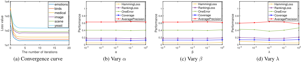
Convergence analysis: Figure 3 (a) shows the convergence curve of the model in multiple data sets. The result shows that with the increase of the number of iterations, the loss value decreases rapidly and finally stabilizes at a low value, indicating that the model converges to a satisfactory solution. Parameter sensitivity analysis: Figure 3 (b), (c) and (d) show the sensitivity experimental results of the three parameters α, β, λ in the model. The results show that each parameter has an optimal value and PML-PLR performs stably across a wide range of parameters, making it capable of robust classification performance under various conditions.
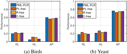
Ablation analysis: Figure 4 shows the ablation results on two datasets, comparing PML-PLR with its three degraded versions: no pseudo-label learning (PL-free, which directly uses candidate labels for classifier training ), no reconstruction (R-free, which sets parameter β=0), and no consistent correlation (C-free, which extracts correlation only from feature matrix X). The results clearly demonstrate that PMLPLR significantly outperforms all degraded algorithms across multiple evaluation metrics, validating the effectiveness and necessity of each component in our proposed framework. The performance drop when removing any single component highlights their complementary nature in addressing the challenges of partial multi-label learning.
| Datasets | PML-PLR | PML-LENFN | PAMB | PML-NI | PARTICLE the better) | FPML | ML-KNN | LIFT |
|---|---|---|---|---|---|---|---|---|
| Ranking | Loss (the smaller | |||||||
| Emotions | 0.166±0.027 | 0.210±0.027 | 0.192±0.032 | 0.263±0.029 | 0.446±0.027 | 0.407±0.014 | 0.249±0.044 | 0.211±0.035 |
| Birds | 0.197±0.032 | 0.200±0.028 | 0.204±0.024 | 0.205±0.034 | 0.326±0.027 | 0.341±0.020 | 0.250±0.041 | 0.214±0.030 |
| Medical | 0.032±0.012 | 0.068±0.021 | 0.113±0.032 | 0.100±0.028 | 0.102±0.018 | 0.059±0.010 | 0.093±0.021 | 0.046±0.010 |
| Image | 0.180±0.018 | 0.212±0.026 | 0.217±0.015 | 0.230±0.024 | 0.261±0.070 | 0.254±0.018 | 0.272±0.023 | 0.235±0.015 |
| Scene | 0.134±0.011 | 0.242±0.018 | 0.250±0.016 | 0.284±0.013 | 0.291±0.130 | 0.153±0.013 | 0.348±0.024 | 0.278±0.018 |
| Yeast | 0.178±0.012 | 0.190±0.016 | 0.211±0.007 | 0.202±0.016 | 0.189±0.009 | 0.191±0.017 | 0.193±0.015 | 0.188±0.011 |
| Health | 0.067±0.003 | 0.076±0.006 | 0.081±0.007 | 0.096±0.007 | 0.110±0.008 | 0.063±0.003 | 0.077±0.004 | 0.070±0.006 |
| Reference | 0.103±0.004 | 0.130±0.009 | 0.110±0.008 | 0.152±0.009 (the | 0.156±0.015 smaller the better) | 0.101±0.005 | 0.116±0.009 | 0.118±0.007 |
| Hamming Loss | ||||||||
| Emotions | 0.214±0.013 | 0.247±0.022 | 0.221±0.022 | 0.500±0.047 | 0.253±0.022 | 0.330±0.013 | 0.261±0.022 | 0.570±0.035 |
| Birds | 0.046±0.004 | 0.093±0.007 | 0.101±0.009 | 0.061±0.011 | 0.149±0.010 | 0.109±0.023 | 0.049±0.006 | 0.051±0.007 |
| Medical | 0.013±0.001 | 0.013±0.003 | 0.025±0.001 | 0.023±0.002 | 0.037±0.003 | 0.015±0.001 | 0.085±0.001 | 0.012±0.002 |
| Image | 0.203±0.009 | 0.215±0.027 | 0.217±0.010 | 0.227±0.015 | 0.236±0.056 | 0.249±0.016 | 0.222±0.015 | 0.572±0.013 |
| Scene | 0.149±0.010 | 0.211±0.017 | 0.203±0.022 | 0.644±0.053 | 0.277±0.002 | 0.158±0.012 | 0.759±0.026 | 0.820±0.003 |
| Yeast | 0.213±0.004 | 0.234±0.012 | 0.215±0.008 | 0.248±0.036 | 0.217±0.008 | 0.232±0.006 | 0.315±0.013 | 0.587±0.008 |
| Health | 0.035±0.001 | 0.038±0.002 | 0.044±0.001 | 0.036±0.002 | 0.051±0.003 | 0.045±0.001 | 0.049±0.001 | 0.047±0.003 |
| Reference | 0.029±0.001 | 0.036±0.002 | 0.036±0.001 | 0.030±0.001 Precision (the | 0.035±0.001 larger the | 0.027±0.001 better) | 0.033±0.001 | 0.037±0.001 |
| Average | ||||||||
| Emotions | 0.792±0.003 | 0.768±0.028 | 0.783±0.036 | 0.749±0.034 | 0.739±0.033 | 0.730±0.016 | 0.720±0.039 | 0.746±0.033 |
| Birds | 0.594±0.032 | 0.581±0.048 | 0.564±0.044 | 0.572±0.041 | 0.419±0.046 | 0.373±0.020 | 0.525±0.062 | 0.550±0.062 |
| Medical | 0.872±0.027 | 0.803±0.031 | 0.725±0.020 | 0.732±0.035 | 0.835±0.024 | 0.822±0.022 | 0.726±0.037 | 0.845±0.018 |
| Image | 0.764±0.009 | 0.747±0.029 | 0.748±0.019 | 0.732±0.024 | 0.725±0.084 | 0.696±0.023 | 0.689±0.022 | 0.720±0.019 |
| Scene | 0.800±0.000 | 0.649±0.025 | 0.722±0.023 | 0.609±0.018 | 0.649±0.149 | 0.753±0.020 | 0.527±0.024 | 0.613±0.027 |
| Yeast | 0.752±0.020 | 0.740±0.017 | 0.753±0.013 | 0.725±0.016 | 0.744±0.011 | 0.730±0.013 | 0.729±0.017 | 0.734±0.014 |
| Health | 0.760±0.008 | 0.750±0.016 | 0.680±0.016 | 0.723±0.018 | 0.501±0.045 | 0.695±0.010 | 0.650±0.012 | 0.716±0.019 |
| Reference | 0.671±0.012 | 0.643±0.012 | 0.612±0.015 | 0.614±0.011 | 0.448±0.058 | 0.576±0.014 | 0.589±0.007 | 0.619±0.014 |
5 Conclusion
This paper presents a novel PML method, PML-PLR, which jointly extracts instance-level correlation from candidate labels and features, and then uses the instance correlation as reconstruction coefficient to reconstruct pseudo-labels. Through local manifold learning, the reconstructed pseudolabels are used to propagate the consistency relationship between labels and instances, thereby improving the accuracy of pseudo-labels. Extensive experiments demonstrate the superiority of the model.
Acknowledgments
This work was supported in part by the National Natural Science Foundation of China under Grant No. 62176065, No. 62302172, in part by the Guangdong Provincial National Science Foundation under Grant No. 2022A1515011277.
@inproceedings{ijcai2025p545,
  title     = {Pseudo-Label Reconstruction for Partial Multi-Label Learning},
  author    = {Chen, Yu and Li, Fang and Han, Na and Li, Guanbin and Gao, Hongbo and Chan, Sixian and Fang, Xiaozhao},
  booktitle = {Proceedings of the Thirty-Fourth International Joint Conference on
               Artificial Intelligence, {IJCAI-25}},
  publisher = {International Joint Conferences on Artificial Intelligence Organization},
  editor    = {James Kwok},
  pages     = {4896--4904},
  year      = {2025},
  month     = {8},
  note      = {Main Track},
  doi       = {10.24963/ijcai.2025/545},
  url       = {https://doi.org/10.24963/ijcai.2025/545},
}
TY - CPAPER TI - Pseudo-Label Reconstruction for Partial Multi-Label Learning AU - Chen, Yu AU - Li, Fang AU - Han, Na AU - Li, Guanbin AU - Gao, Hongbo AU - Chan, Sixian AU - Fang, Xiaozhao T2 - Proceedings of the Thirty-Fourth International Joint Conference on Artificial Intelligence, IJCAI-25 PB - International Joint Conferences on Artificial Intelligence Organization PY - 2025 SP - 4896 EP - 4904 DO - 10.24963/ijcai.2025/545 UR - https://doi.org/10.24963/ijcai.2025/545 ER -Copied
Machine-readable versions of this paper, for tools and AI agents:





