
An Inverse Optimization Approach to Contextual Inverse Optimization
Proceedings of the Thirty-Fourth International Joint Conference on Artificial Intelligence. Main Track. Pages 5354-5362.
https://doi.org/10.24963/ijcai.2025/596
Keywords
- Machine Learning: ML: Supervised Learning
- Machine Learning: ML: Optimization
- Constraint Satisfaction and Optimization: CSO: Mixed discrete and continuous optimization
Abstract
Contextual Inverse Optimization (CIO) is a generalized framework of the predict-then-optimize approach, also referred to as decision-focused learning or contextual optimization, aiming to learn a model that predicts the unknown parameters of a nominal optimization problem using related covariates without compromising the solution quality. Unlike the predict-then-optimize approach, which assumes access to datasets containing realized unknown parameters, CIO considers a setting where only historical optimal solutions are available. Previous work has primarily focused on CIO under linear programming problems and proposed methods based on optimality conditions. In this study, we propose a general algorithm based on inverse optimization as a more general approach that does not require optimality conditions. To validate its effectiveness, we apply the proposed method to multiple CIO problems and demonstrate that it performs comparably to or better than existing predict-then-optimize methods, even without ground-truth unknown parameters.
- [Ahuja and Orlin, 2000] Ravindra K Ahuja and James B Or- lin. A faster algorithm for the inverse spanning tree prob- lem. Journal of Algorithms, 34(1):177-193, 2000.
- [Amos and Kolter, 2017] Brandon Amos and J. Zico Kolter. OptNet: Differentiable optimization as a layer in neural networks. In Proceedings of the 34th International Con- ference on Machine Learning, volume 70 of Proceedings of Machine Learning Research, pages 136-145. PMLR, 2017.
- [Berthet et al., 2020] Quentin Berthet, Mathieu Blondel, Olivier Teboul, Marco Cuturi, Jean-Philippe Vert, and Francis Bach. Learning with differentiable pertubed op- timizers. In H. Larochelle, M. Ranzato, R. Hadsell, M.F. Balcan, and H. Lin, editors, Advances in Neural Informa- tion Processing Systems, volume 33, pages 9508-9519.
- Curran Associates, Inc., 2020.
- [Bertsimas and Kallus, 2020] Dimitris Bertsimas and Nathan Kallus. From predictive to prescriptive analytics. Management Science, 66(3):1025-1044, March 2020.
- [Besbes et al., 2023] Omar Besbes, Yuri Fonseca, and Ilan Lobel. Contextual inverse optimization: Offline and online learning. Operations Research, August 2023.
- [Blondel, 2019] Mathieu Blondel. Structured prediction with projection oracles. In Hanna M. Wallach, Hugo Larochelle, Alina Beygelzimer, Florence d'Alché-Buc, Emily B. Fox, and Roman Garnett, editors, Advances in Neural Information Processing Systems 32: Annual Con- ference on Neural Information Processing Systems 2019, NeurIPS 2019, December 8-14, 2019, Vancouver, BC, Canada, pages 12145-12156, 2019.
- [Bodur et al., 2022] Merve Bodur, Timothy CY Chan, and Ian Yihang Zhu. Inverse mixed integer optimization: Poly- hedral insights and trust region methods. INFORMS Jour- nal on Computing, 34(3):1471-1488, 2022.
- [Bulut and Ralphs, 2021] Aykut Bulut and Ted K. Ralphs. On the complexity of inverse mixed integer linear opti- mization. SIAM Journal on Optimization, 31(4):3014- 3043, January 2021.
- [Burton and Toint, 1992] D. Burton and Ph. L. Toint. On an instance of the inverse shortest paths problem. Mathemat- ical Programming, 53(1-3):45-61, January 1992.
- [Call and Holmberg, 2011] Mikael Call and Kaj Holmberg. Complexity of inverse shortest path routing. In Network Optimization, pages 339-353. Springer Berlin Heidelberg, 2011.
- [El Balghiti et al., 2019] Othman El Balghiti, Adam N. El- machtoub, Paul Grigas, and Ambuj Tewari. Generaliza- tion bounds in the predict-then-optimize framework. In Advances in Neural Information Processing Systems, vol- ume 32.
- Curran Associates, Inc., 2019.
- [Elmachtoub and Grigas, 2022] Adam N. Elmachtoub and Paul Grigas. Smart "predict, then optimize". Management Science, 68(1):9-26, January 2022.
- [Ferber et al., 2020] Aaron Ferber, Bryan Wilder, Bistra Dilkina, and Milind Tambe. Mipaal: Mixed integer pro- gram as a layer. Proceedings of the AAAI Conference on Artificial Intelligence, 34(02):1504-1511, April 2020.
- Gurobi Optimization, LLC. Gurobi Optimizer Reference Manual, 2024.
- [Heuberger, 2004] Clemens Heuberger. Inverse combinato- rial optimization: A survey on problems, methods, and re- sults. Journal of Combinatorial Optimization, 8(3):329- 361, September 2004.
- [Hu et al., 2022] Yichun Hu, Nathan Kallus, and Xiaojie Mao. Fast rates for contextual linear optimization. Man- agement Science, 68(6):4236-4245, June 2022.
- [Huang and Liu, 1999] Siming Huang and Zhenhong Liu. On the inverse problem of linear programming and its ap- plication to minimum weight perfect k-matching1research supported in part by a grant from hong kong university of science and technology through dag92/93.bm15.1. Euro- pean Journal of Operational Research, 112(2):421-426, 1999.
- [Kingma and Ba, 2014] Diederik P. Kingma and Jimmy Ba. Adam: A method for stochastic optimization. 2014.
- [Luenberger and Ye, 2008] David G. Luenberger and Yinyu Ye. Linear and Nonlinear Programming. Springer US, 2008.
- [Mandi et al., 2022] Jayanta Mandi, Víctor Bucarey, Maxime Mulamba Ke Tchomba, and Tias Guns. Decision-focused learning: Through the lens of learning to rank. In International Conference on Machine Learn- ing, ICML 2022, 17-23 July 2022, Baltimore, Maryland, USA, volume 162 of Proceedings of Machine Learning Research, pages 14935-14947. PMLR, 2022.
- [Mandi et al., 2024] Jayanta Mandi, James Kotary, Senne Berden, Maxime Mulamba, Victor Bucarey, Tias Guns, and Ferdinando Fioretto. Decision-focused learning: Foundations, state of the art, benchmark and future oppor- tunities. Journal of Artificial Intelligence Research, 2024.
- [Mishra et al., 2024] Saurabh kumar Mishra, Anant Raj, and Sharan Vaswani. From inverse optimization to feasibility to ERM. In Forty-first International Conference on Ma- chine Learning, 2024.
- [Mulamba et al., 2021] Maxime Mulamba, Jayanta Mandi, Michelangelo Diligenti, Michele Lombardi, Victor Bu- carey, and Tias Guns. Contrastive losses and solution caching for predict-and-optimize. In Zhi-Hua Zhou, ed- itor, Proceedings of the Thirtieth International Joint Con- ference on Artificial Intelligence, IJCAI-21, pages 2833- 2840. International Joint Conferences on Artificial Intelli- gence Organization, 8 2021. Main Track. IJCAI
- [Roland et al., 2013] Julien Roland, José Rui Figueira, and Yves De Smet. The inverse {0, 1}-knapsack problem: Theory, algorithms and computational experiments. Dis- crete Optimization, 10(2):181-192, 2013.
- [Sadana et al., 2024] Utsav Sadana, Abhilash Chenreddy, Erick Delage, Alexandre Forel, Emma Frejinger, and Thibaut Vidal. A survey of contextual optimization meth- ods for decision-making under uncertainty. European Journal of Operational Research, 2024.
- [Schaefer, 2009] Andrew J. Schaefer. Inverse integer pro- gramming. Optimization Letters, 3(4):483-489, June 2009.
- [Sen et al., 2008] Prithviraj Sen, Galileo Namata, Mustafa Bilgic, Lise Getoor, Brian Gallagher, and Tina Eliassi- Rad. Collective classification in network data. AI Mag- azine, 29(3):93-106, September 2008.
- [Sun et al., 2023] Chunlin Sun, Shang Liu, and Xiaocheng Li. Maximum optimality margin: A unified approach for contextual linear programming and inverse linear programming. In International Conference on Ma- chine Learning, ICML 2023, 23-29 July 2023, Honolulu, Hawaii, USA, volume 202 of Proceedings of Machine Learning Research, pages 32886-32912.
- PMLR, 2023.
- [Tang and Khalil, 2024] Bo Tang and Elias B. Khalil. Pyepo: a pytorch-based end-to-end predict-then-optimize library for linear and integer programming. Mathematical Pro- gramming Computation, July 2024. Vlastelica et al., 2020]
- Marin Vlastelica, Anselm Paulus, Vít Musil, Georg Martius, and Michal Rolínek. Differen- tiation of blackbox combinatorial solvers. In International Conference on Learning Representations, 2020.
- [Wang, 2009] Lizhi Wang. Cutting plane algorithms for the inverse mixed integer linear programming problem. Oper- ations Research Letters, 37(2):114-116, 2009.
- [Wang, 2013] Lizhi Wang. Branch-and-bound algorithms for the partial inverse mixed integer linear programming problem. Journal of Global Optimization, 55(3):491-506, 2013.
- [Wilder et al., 2019] Bryan Wilder, Bistra Dilkina, and Milind Tambe. Melding the data-decisions pipeline: Decision-focused learning for combinatorial optimization. Proceedings of the AAAI Conference on Artificial Intelli- gence, 33(01):1658-1665, July 2019.
- [Zhang et al., 1999] Jianzhong Zhang, Zhenhong Liu, and Zhongfan Ma. The inverse fractional matching problem. The Journal of the Australian Mathematical Society. Se- ries B. Applied Mathematics, 40(4):484-496, 1999.
References were extracted automatically from the PDF and may contain errors.
Full text extracted automatically from the PDF; figures, tables and equations may differ. The PDF is the version of record.
1 Introduction
In many decision-making problems modeled as optimization problems, a decision-maker frequently suffers from the fact that some parameters of the optimization model contain uncertainty. For instance, a road planner predicts traffic demand based on information about weather conditions or time of day and presents an optimal route to drivers based on the forecast results. The predict-then-optimize paradigm [El Balghiti et al., 2019; Elmachtoub and Grigas, 2022] studies a setting where the decision-maker has access to a history of covariates which is correlated with the unknown parameter of the optimization model and the realization of the unknown parameters in the past, and the objective is to learn a model that predicts unknown parameters which leads to a better quality of decisions.
One might think that it is sufficient to build a prediction model by using existing statistical or machine learning methods, such as ridge regression, and then subsequently perform an optimization process with the output of the trained model.
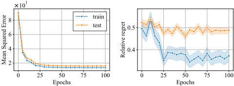
Figure 1 shows that such a typical two-stage framework fails to produce a high-quality decision. On the left-hand side of Figure 1, the history of the mean squared loss is shown for predicting the coefficient vector of the shortest path problem. The right-hand side of Figure 1 shows a history of relative regrets, which represents the difference between the true optimal value and the objective value calculated by the solution of an optimization problem whose unknown parameters are predicted by a trained model. It can be observed that a model trained using the mean squared error does not significantly contribute to improving the solution quality. Indeed, the regret on the test data (orange line) shows little improvement from the initial parameters.
Besides a predict-then-optimize paradigm, methodologies to support high-quality decision-making in the presence of uncertainty by integrating machine learning and optimization methods have been extensively studied in the name of contextual optimization [Hu et al., 2022; Sadana et al., 2024], decision-focused learning [Amos and Kolter, 2017; Wilder et al., 2019; Mandi et al., 2022] and prescriptive analysis [Bertsimas and Kallus, 2020].
The paradigms mentioned above consider a situation in which the available data contains the realized unknown optimization parameters to be predicted. In contrast, research on what is called contextual inverse optimization, which considers a more general situation in which the realized optimal solutions to the nominal optimization problem of interest are available, has attracted much attention [Sun et al., 2023; Besbes et al., 2023; Mishra et al., 2024].
Prior work on contextual inverse optimization [Sun et al., 2023; Mishra et al., 2024] has basically focused on linear programming problems and proposed learning methods based on the optimality conditions. These methods are fundamentally limited to linear programming problems to which optimality conditions can be applicable, and cannot be directly applied to more general problems, such as integer programming problems, where the feasible region is defined as a subspace of discrete space.
In this paper, to address the limitation of the optimization problem that can be handled in the existing methods for contextual inverse optimization, we propose a general method for solving contextual inverse optimization problems involving integer programming problems that do not explicitly require the optimality conditions.
1.1 Contributions
The contributions of this study are summarized as follows:
- We provide a method for solving contextual inverse optimization problems. Unlike existing work for contextual inverse optimization [Sun et al., 2023; Mishra et al., 2024], the proposed method is not limited to linear programs and can be applied to any linear objective optimization problem, including integer programs in which inverse optimization can be applicable. Furthermore, unlike existing predict-then-optimize methods, our method does not require hyperparameter tuning for the learning rate. As a result, the model can be trained in fewer epochs compared to traditional methods.
- The proposed method employs an inverse optimization algorithm as an oracle. This study demonstrates that inverse optimization can be effectively utilized as an algorithm for contextual inverse optimization problems. It is known that inverse optimization can be efficiently solved for specific problems like the knapsack problem. As algorithms for inverse optimization continue to advance, it is expected that the proposed method will also improve.
- We empirically examine the effectiveness of the proposed method for several contextual integer optimization problems. Although our method does not need the ground-truth unknown parameters of the nominal optimization problem, the performance is competitive with existing methods such as smart, predict-then-optimize [El Balghiti et al., 2019] that require the unknown parameters and perturbed-based method [Berthet et al., 2020]. Additionally, while the proposed method requires more computation time per iteration than existing methods, we found that the overall computational time is comparable with that of existing methods because it converges after a small number of iterations.
1.2 Notation
Let n be a positive integer. Define N as a set of positive integers. Let Rn and Zn be the set of real-valued vectors of dimension n and the set of integer vectors of dimension n, respectively. Additionally, let Rn+ and Zn+ be a set of nonnegative real-valued vectors of dimension n and a set of nonnegative integer vectors of dimension n, respectively. Let [n] be a finite set {1, 2, . . . , n}. We use lowercase bold letters for vectors and uppercase bold letters for matrices. Let In be an identity matrix of size n and O be a zero matrix of appropriate size. For a vector x ∈ Rn , the symbol ∥·∥ denotes a general norm on Rn , ∥·∥p denotes the p-norm for p ≥ 1 on Rn , and ∥·∥∞ denotes the maximum norm on Rn .
2 Problem Statement
Let n and d be positive integers. Given a feasible region X ⊆ Zn , consider an integer programming problem 1 (IP) which is formulated as follows:
where x ∈ X is a decision variable and c ∈ C is an unknown parameter vector. Here, C ⊆ Rn is a domain in which the vector c lives. Let x⋆ (c) ∈ X be an optimal solution to the IP(c,X). The exact value of a vector c is not known in advance, but a covariate z ∈ Rd correlated with c is available. In other words, we have access to a historical dataset DN = {(zi, x⋆i )}Ni=1 , which consists of a pair of a covariate and an optimal solution. Here, for any i ∈ [N], x⋆i is an optimal solution to the IP(ci, X), where ci is the true cost vector realized when the covariate is zi.
In contrast to the predict-then-optimize setting, the contextual inverse optimization setting is more challenging because true cost vectors are not included in the dataset. Thus, even simple two-stage methods cannot be directly applied. Indeed, the predict-then-optimize setting can be reduced to the contextual inverse optimization setting by solving the optimization problem for the true cost vectors included in the dataset.
The primary objective of the contextual inverse optimization setting is to obtain a prediction model that maps a covariate to an unknown coefficient vector of a nominal optimization problem, which leads to a quality decision. Denote the prediction model by f(·;Θ) : Rd → C where Θ is a model parameter to be trained by some methods.
In the typical supervised learning setting, the performance metric is considered how close the predicted cost cpred = f(z;Θ) is to the true cost c. However, in the problem setting described above, the ultimate goal is to obtain an optimal solution x⋆ (cpred) that is close to the optimal solution x⋆ (c). To measure how well the prediction model performs, the regret for the maximization problem in Eq. (1) is defined as
which measures the difference between the optimal objective value c⊤x⋆ (c) and the objective value c⊤x⋆ (cpred) when the decision is x⋆ (cpred) with ground truth c. Note that the metric becomes 0 when the optimal solution with the predicted cost vector is identical to that of the true optimal solution.
1 This study can naturally be extended to mixed-integer linear programming problems; however, in this paper, we focus on integer programming problems.
3 Algorithm
Denote the integer programming problem of interest by IP(c,X) formulated in Eq. (1) where X ⊆ Zn is a feasible region and c ∈ Rn is a cost vector of the objective function. Let x0 ∈ X be a feasible solution to the problem IP(c,X). For a reference vector r ∈ Rn , the inverse optimization problem is defined as the following optimization problem:
Notice that the optimal solution to the above optimization problem in Eq. (3) determines the optimal profit vector q⋆ that minimizes the distance from a given r with respect to a norm ∥·∥ such that a given feasible solution x0 be an optimal solution to the modified optimization problem IP(q⋆ , X ).
Using an available dataset DN = {(zi, x⋆i )}Ni=1 , we aim to find a model parameter Θ⋆ so that the optimal solution to IP(̂ cnew, X), where ̂ cnew = f(znew;Θ⋆ ), is close to the optimal solution to IP(cnew, X). Here, znew is a new observation of the context, and cnew is a ground-truth cost vector of IP of interest. In light of the above, for each data point (zi, x⋆i ), we first predict a cost vector by the current model ̂ ci = f(zi;Θ) and obtain a perturbed vector ˜ ci,k = ̂ ci + εk where εk ∼ N(0, σIn) for some σ > 0 and k = 1, 2, . . . ,M. Then, we solve the inverse optimization problem in Eq. (3) for each perturbed cost vector, and obtain their solutions ˜ qi,k for k ∈ [M]. Finally, we update the current model parameter as the optimal solution to the following optimization problem:
where {˜ qi,k}i∈[N],k∈[M] ⊆ Rn are optimal solutions to IOP(˜ ci,k, x⋆ , ∥·∥) for some norm ∥·∥ in Eq. (3). We present the pseudocode of the proposed algorithm to solve the contextual inverse optimization in Algorithm 1.
The proposed update rule in Eq. (4) is related to minimize the loss function defined by ℓ(Θ) := E(z,x)∼P [h(Θ; z, x)] where h(Θ; z, x) := 1 2 Eq(x)∼Px [∥f (z; Θ) - q(x)∥22 ]. Here, P and Px denote the underlying distribution of the data and the distribution on the set of all coefficient vectors whose optimal solution to IP(c,X) is x, respectively. By minimizing ℓ(Θ), it is expected that minimizing the model parameter Θ can be obtained to prescribe a high-quality solution based on the new context z.
3.1 Linear Model Case
We discuss the case of a linear model f(z;Θ) = zΘ where z ∈ R1×d . Let L(Θ) be an objective function of the convex quadratic optimization problem in Eq. (4). Taking gradient of the objective function of the problem in Eq. (4), L(Θ), with respect to Θ, we have
Algorithm 1: Algorithm for Contextual Inverse Optimization Problem (full batch size)
Define qi := 1M ∑Mk=1 ˜ qi,k. Then, by introducing matrices Z := [z⊤ 1 , z⊤ 2 , . . . , z⊤ N ]⊤ ∈ RN×d and Q = [q1, q2, . . . , qN] ∈ Rn×N , we have
By solving a linear system ∇ΘL(Θ) = O under the condition that Z⊤Z is invertible, we have the following closed form for the optimization problem of Eq. (4):
Unlike learning-based methods, the proposed method does not require setting a learning rate, which eliminates the need for hyperparameter tuning. Algorithm 1 has two parameters, M and σ, but we confirm that setting both to 1 achieves sufficiently high performance in Section 4.
3.2 Inverse Integer Programming Problem
To implement Algorithm 1, it is necessary to have an inverse optimization oracle IOP(·, ·, ∥·∥) for some norm ∥·∥. Below, we review the prior work on solving inverse problems for integer programs [Ahuja and Orlin, 2000; Heuberger, 2004].
The inverse integer programming problems under ℓ1 norm are known to be reformulated into a linear programming problem [Schaefer, 2009]. However, the number of both decision variables and constants grows exponentially, which makes it impractical to solve in a realistic time. It has been shown in [Wang, 2009] and [Bulut and Ralphs, 2021] that inverse integer programming problems can be solved by a cutting-plane method. Given x0 and a reference point r, the cutting-plane algorithm solves the following problem at the tth iteration:minimize
where Et = {x1 , x2 , . . . , xt} is the optimal solutions generated in the previous iterations so far. After obtaining the Algorithm 2: A Cutting-Plane Algorithm for Inverse Integer Programming Problem (c.f., [Wang, 2009])
Input: Integer program IP(c,X), feasible solution x0 ∈ X , and reference point r.
Output: Cost vector q such that the optimal solution to revised problem IP(q, X) is x0 .
- 1 Initialization: Set q1 = r, x1 be an optimal solution to problem in Eq. (7), E1 ← {x1}, and t ← 1.
3 Solve optimization problem (6) and obtain qt.
4 Solve integer program (7) and obtain xt.
- 5 Update Et+1 ← Et ∪ {xt} and t ← t +1.
- 6 return qt.
optimal solution qt to the problem (6), the algorithm solves the following integer programming problem:
If the condition q⊤ t (xt -x0 ) ≤ 0 satisfies, then the algorithm terminates and outputs qt as an optimal solution to the inverse optimization problem; otherwise update Et+1 = Et ∪ {xt } and repeat the above procedure. We present the pseudo-code of the cutting plane algorithm in 2. It has been proven that Algorithm 2 terminates in a finite number of iterations and outputs an optimal solution to the inverse integer programming problem [Wang, 2009, Theorem 1, Theorem 2].
Note that inverse optimization for mixed-integer programming problems has also been studied, and algorithms based on the branch-and-bound [Wang, 2013] and cutting-plane method [Bulut and Ralphs, 2021; Bodur et al., 2022] have been proposed. Thus, the proposed method can be naturally extended to solve contextual inverse mixed-integer programming problems.
3.3 Inverse Optimization of Specific Problems
In Section 3.2, we have discussed that any inverse optimization problems can be solved by the cutting-plane algorithm. However, the cutting-plane algorithmmay not be efficient because it requires solving optimization problems iteratively as a subproblem at each iteration (c.f., line 3 and 4 in Algorithm 2). In this subsection, we discuss that inverse optimization problems can be solved more efficiently by considering the specific structure of the target optimization problem. Here, we take the {0, 1}-knapsack problem as an example [Roland et al., 2013], but other optimization problems, such as shortest path problems [Burton and Toint, 1992; Call and Holmberg, 2011] and matching problems [Zhang et al., 1999; Huang and Liu, 1999], have also been studied. It should be mentioned that the knapsack problem is an important combinatorial optimization problem because it can be used to model resource allocation under constraints, providing a foundation for optimizing decisions in finance, logistics, and scheduling through combinatorial optimization techniques.
Consider the {0, 1}-knapsack problem in which a decision maker selects a pair of given n items numbered as I = [n]
with the aim of maximizing the sum of utility under a capacity constraint. Formally, the {0, 1}-knapsack problem is formulated as follows:
where c = (ci)ni=1 is a utility of items, w = (wi)ni=1 is items weights, and W ∈ N is a maximum weight capacity.
Let gi(µ) ∈ R be the maximum utility that can be achieved when considering the first i items of the set of items I and a capacity µ ∈ {0, 1, . . . ,W}. The value of gi(u) can be determined through the optimal value of the following combinatorial optimization problem:
The optimal value to the original {0, 1}-knapsack problem in Eq. (8) is equivalent to finding the value of gn(W). Notice that the {0, 1}-knapsack problem can be solved by the dynamic programming formulated as
with the initial state g1(µ) = 0 for µ ∈ {0, 1, . . . ,w1 -1} and g1(µ) = c1 for µ ∈ {w1,w1 +1, . . . ,W}. This dynamic programming approach can be reduced to a linear programming problem to minimize gn(W) under the set of linear constraints of gi(µ) for i ∈ [n], µ ∈ {0, 1, . . . ,W}. For a given feasible solution x0 ∈ Rn and a reference point r ∈ Rn , [Roland et al., 2013] has shown that the following linear programming problem finds a vector d⋆ ∈ Rn+ with (q⋆ )⊤x0 = max {(q⋆ )⊤x ∣∣ x ∈ X } under some norm ∥·∥:
where q ∈ Rn+ and (gi(µ))i,µ are decision variables. In case we take ∥·∥ as ℓ1 norm or ℓ∞ norm, the above problem is reduced to be a linear programming problem.
4 Numerical Experiments
To investigate the effectiveness of the proposed method, we conducted numerical experiments on several optimization problems and compared the proposed method against the existing methods for a predict-then-optimize framework.
Specifically, we consider the {0, 1}-knapsack problem formulated in Eq. (8) and the diverse bipartite matching problem adapted in [Ferber et al., 2020] following the synthetic data generation process studied in [Elmachtoub and Grigas, 2022]. As for existing methods, we employed a ridge regression as a two-stage approach (2s), smart predict-then-optimize (spo+) [Elmachtoub and Grigas, 2022], differentiation of black box combinatorial solvers (dbb) [Vlastelica et al., 2020], a noise contrastive estimation approach (nce) [Mulamba et al., 2021], a learning to rank approach (ltr) [Mandi et al., 2022], and a perturbed optimizers approach (pfy) [Berthet et al., 2020].
We implemented all the existing methods by using the pyepo package [Tang and Khalil, 2024] and trained all the methods for 100 number of epochs with the full batch size. For existing methods, we employed Adam optimizer [Kingma and Ba, 2014] with a learning rate η = 10-2 to minimize each loss function. For the learning to rank methods, we employed pairwise loss and listwise loss, and we set the ratio of calling the optimization oracle as 0.5. For the perturbed optimizer approach, we set both the number of perturbations and the amplitude of the perturbation as 1. For the proposed method (Algorithm 1), we set T = 100, M = 1, σ = 1, and we solve the inverse optimization problem by the optimization problem given in Eq. (10) for a {0, 1}- knapsack problem and the cutting-plane algorithm (Algorithm 2) for a diverse bipartite matching problem. For both methods, we use the linear model, f(z;Θ) = zΘ, to predict a coefficient vector.
It should be mentioned that several approaches to contextual inverse optimization problems have been proposed [Sun et al., 2023; Mishra et al., 2024]; however, these methods are limited to linear programming problems (and quadratic programs) to which optimality conditions can be exploited, and thus we excluded these methods in this experiment.
Experimental programs were implemented in Python 3.11 and run on a Windows 10 PC with an Intel(R) Xeon(R) W1270 CPU 3.40 GHz and 64 GB RAM. For both the existing and proposed methods, we used the Gurobi Optimizer 11.0.2 [Gurobi Optimization, LLC, 2024] to solve the optimization problems.
4.1 ProblemDescription
Since we have already described the {0, 1}-knapsack problem in Section 3.3, we omit the problem description here. We present the problem definition of the diverse bipartite matching problem adapted in [Ferber et al., 2020], in which the objective is to find an optimal matching between the scientific publications with the desired proportion. This problem is formulated as the following integer programming problem:
where N1 and N2 are the sets of nodes representing scientific publications, X(m, p, q) is a feasible set, and c = (ci,j)∀i∈N1,∀j∈N2 is a reward matrix which indicates the likelihood that a link between each pair of nodes from N1 to N2 exists. Also, m = (mi,j)∀i∈N1,∀j∈N2 is a binary matrix indicating the relationship between publications, and p, q ∈ [0, 1]
are proportions of sharing each field. The formal description of the constraints is referred to [Ferber et al., 2020].
4.2 Synthetic Data Generation
Next, we provide the synthetic data generation process for the optimization problems to be solved. A vector of a covariate z ∈ Rd is generated from the normal distribution N(µ, σ2 ) with a mean µ = 0 and variance σ2 = 1, and a coefficient vector c ∈ Rn is generated from a polynomial mapping from the covariates with additional noise. Formally, each element of the cost vector is generated as per the following model:
where deg > 0 is a fixed positive integer representing a polynomial degree, B⋆ ∈ Rn×d is a latent true coefficient matrix whose each entry B⋆ kl (k ∈ [n], l ∈ [d]) takes 1 with probability 0.5 and 0 with probability 0.5, and εj is a multiplicative noise term that is sampled from the uniform distribution on [1 - ε, 1 + ε] for some constant parameter ε > 0.
For the {0, 1}-knapsack problem in Eq. (8), we set the dimensionality of the covariates as d = 5, the number of items as n = 20, and the maximum capacity of the knapsack as W = 30. The utility vector of each item c is generated according to the polynomial model in Eq. (12). The weights of each item are generated as wi = ⌊ 1 100 ui⌋ where ui ∼ Unif({300, 301, . . . , 799}).
For the diverse bipartite matching problem in Eq. (11), we set the dimensionality of the covariates as d = 5, the number of nodes in N1 and N2 as |N1| = |N2| = 5, the desired proportion as p = q = 0.25, and the reward matrix c is generated according to the polynomial model in Eq. (12). Note that the original bipartite matching problem [Ferber et al., 2020] is formulated on graphs sampled from the CORA citation network dataset [Sen et al., 2008], but we consider the synthetic data generation process because the size of the original optimization problem is large, so that the proposed method does not work in realistic time.
For the experiments, we first construct a dataset consists of ˜DN = {(zi, ci, x⋆i )}Ni=1 where {zi}Ni=1 and {ci}Ni=1 are generated by the above procedure, and {x⋆i }Ni=1 are the optimal solutions to the optimization problem of interest when the unknown parameters are given by {ci}Ni=1 . Existing predict-then-optimize methods require DN = {(zi, ci)}Ni=1 as the dataset, whereas our method only require DN = {(zi, x⋆i )}Ni=1 . For all experiments, we set the number of training samples as N = 1000 and the number of test samples as N = 1000.
4.3 Performance Metrics
In this numerical experiment, especially for a maximization problem, we consider relative regret as a performance measure. For the predicted coefficient vector ̂ c of the objective function, the relative regret is defined as
where c and x⋆ (·) are the true coefficient vector and the optimal solution, respectively. For the dataset ˜DN, we report the average and standard deviation of the relative regret.
4.4 Results
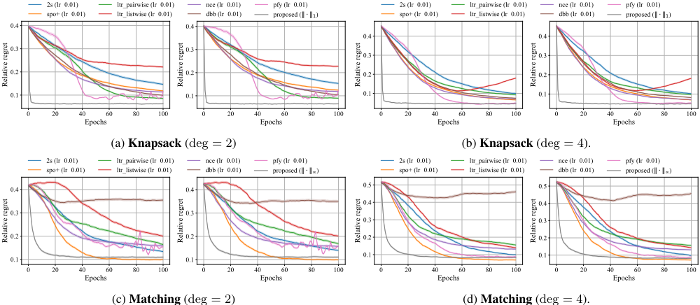
Performance In Figure 2, we show the history of an average of relative regret in Eq. (13) for each method to the {0, 1}- knapsack problem with a polynomial degree deg ∈ {2, 4} (Figures (2a,2b)) and the diverse bipartite matching problem with deg ∈ {2, 4} (Figures (2c, 2d)), respectively. The error bands represent an interval ±1 of the standard deviation from the average. Regarding the proposed method, we report the results of Algorithm 1 with IOP(·, ·, ∥·∥1) for the {0, 1}- knapsack problem, and Algorithm 1 with IOP(·, ·, ∥·∥∞) for the diverse bipartite matching problem.
As an overall trend, we can see that the proposed method shows a rapid decrease in relative regret in the early stages of learning compared to other predict-then-optimize methods. This is because the proposed method is not a learningbased method, and thus it does not require the learning rate tuning. Among the existing methods, spo+ and pfy perform well, which is consistent with the results reported in numerical experiments in prior work (e.g., [Mandi et al., 2022; Sun et al., 2023; Mishra et al., 2024]). spo+ is the best for the diverse bipartite matching problem. In addition, pfy shows good performance, but the results show unstable when deg = 2 for both problems. Finally, we emphasize again that our proposed method does not need information about the true cost vectors, unlike all other predict-then-optimize methods, except for the perturbed method. Nevertheless, it is remarkable that the proposed method is competitive with the baseline methods.
Computational time From Figure 2, we observe that the proposed method performs as well as or better than existing methods. However, the proposed method needs to solve an inverse optimization problem at each epoch, which is expected to result in higher computational costs compared to existing methods. Therefore, we summarized the computational time per epoch in seconds for each method in Table 1. Although the proposed method incurs several tens of times the computational cost compared to existing methods, it has the advantage of demonstrating high performance in the early stages of training, as shown in Figure 2.
Effect of M in Algorithm 1 So far, we have reported the results of the proposed method with parameter M = 1. Here, we examine how Algorithm 1 performs across different values of M. In this experiment, we set the maximum number of epochs as T = 10. Table 2 presents the mean and standard deviation of the relative regret, and the computational time per epoch for the proposed method with M set to 1, 2, 5, and 10. The results demonstrate that increasing the value of M does not significantly change the performance of the resulting model, which suggests that setting M = 1 is sufficient for practical applications.
5 RelatedWork
This section provides related work that aims to incorporate contextual information about a nominal optimization problem into the learning process for a prediction model. We review the methods for contextual inverse optimization. For a comprehensive overview of contextual optimization and decisionfocused learning, we refer the reader to review papers [Mandi et al., 2024; Sadana et al., 2024].
Contextual inverse optimization is a field that aims to learn a prediction model for unknown parameters of nominal optimization problems using only a historical dataset containing contextual information and corresponding optimal solutions. This framework generalizes contextual optimization, where the historical dataset contains ground-truth unknown parameters that need to be predicted.
| Existing methods | Algorithm 1 | |||||||||
|---|---|---|---|---|---|---|---|---|---|---|
| Problem | 2s | spo+ | ltr (pairwise) | ltr (listwise) | nce | dbb | pfy | ∥·∥1 | ∥·∥2 | ∥·∥∞ |
| Knapsack | 1.78 | 2.33 | 14.17 | 2.21 | 2.17 | 3.16 | 2.44 | 52.80 | 87.71 | 59.90 |
| (0.20) | (0.18) | (3.79) | (0.38) | (0.41) | (0.19) | (0.18) | (22.51) | (30.00) | (39.26) | |
| Matching | 12.03 | 17.89 | 16.68 | 14.66 | 15.01 | 23.73 | 19.22 | 147.15 | 135.14 | 87.11 |
| (1.25) | (1.30) | (3.53) | (3.22) | (3.26) | (1.28) | (1.57) | (18.27) | (19.46) | (14.33) | |
| Algorithm 1 with IOP(·, ·.∥·∥1) | Algorithm 1 with IOP(·, ·.∥·∥2) | Algorithm 1 with IOP(·, ·, ∥·∥∞) | |||||
|---|---|---|---|---|---|---|---|
| Problem | M | Rel-Regret | CPU time (s) | Rel-Regret | CPU time (s) | Rel-Regret | CPU time (s) |
| Knapsack | 1 | 9.80e-02 | 59.1 | 1.02e-01 | 65.5 | 1.09e-01 | 38.4 |
| (4.78e-02) | (47.4) | (4.79e-02) | (3.2) | (5.03e-02) | (2.4) | ||
| 2 | 9.86e-02 | 104.0 | 1.03e-01 | 116.2 | 1.08e-01 | 106.1 | |
| (4.72e-02) | (86.4) | (4.64e-02) | (5.7) | (4.76e-02) | (72.1) | ||
| 5 | 9.64e-02 | 175.2 | 1.00e-01 | 283.6 | 1.07e-01 | 152.8 | |
| (4.78e-02) | (17.1) | (4.62e-02) | (14.6) | (4.80e-02) | (6.7) | ||
| 10 | 9.69e-02 | 445.3 | 1.02e-01 | 615.5 | 1.09e-01 | 364.1 | |
| (4.68e-02) | (38.1) | (4.64e-02) | (17.5) | (4.80e-02) | (15.7) | ||
For contextual inverse linear programming problems, [Sun et al., 2023] proposed a learning method referred to as maximum optimality margin, which is based on the reduced cost optimality condition [Luenberger and Ye, 2008] under the assumption that the target linear program is non-degenerate. Although any linear programming problems can be converted to non-generate problems by adding an arbitrarily small perturbation as the authors of [Sun et al., 2023] have remarked, it is not trivial that the optimal basis and its complement can be obtained by the given optimal solution. Subsequently, [Mishra et al., 2024] proposed a method of alternating projections onto convex sets that employs the Karush-Kuhn-Tucker (KKT) condition for linear programs. They constructed the convex set C such that the given optimal solution x⋆ is an optimal solution to the linear program whose coefficient vector belongs to the element of C. This approach enables us to apply it to general contextual linear optimization problems.
Exceptionally, [Berthet et al., 2020] studied a general framework for transforming discrete optimizations into differentiable operations based on stochastic smoothing to prevent the machine learning pipeline from being broken by discrete decisions. Unlike other research on contextual inverse optimization, this framework can be applied as learning method for arbitrary contextual inverse optimization with a linear objective function. This study also shows the connection with Fenchel-Young losses studied in [Blondel, 2019].
6 Concluding Remarks
In this paper, we have proposed a general method for solving contextual inverse optimization problems. The proposed method is not limited to linear programming problems as studied in prior work [Sun et al., 2023; Mishra et al., 2024], and can be applied to any linear objective optimization problems, including integer programming problems in which inverse optimization can be employed. We have shown that the proposed algorithm corresponds to an algorithm that minimizes the loss function with respect to solution quality. Moreover, we have demonstrated the effectiveness of the proposed method for several contextual inverse optimization problems, and the results imply that the performance of the proposed method is competitive with existing predict-then-optimize methods including SPO [Elmachtoub and Grigas, 2022] even though our method does not need the ground-truth unknown parameters of the nominal optimization problem.
For future work, we would like to mention three directions. First, the proposed method requires solving inverse optimization problems exactly, which poses a challenge in terms of scalability. Therefore, we are interested in developing fast algorithms to solve inverse optimization through relaxation or other techniques. Second, it would be interesting to extend a theoretical analysis of the proposed method. Specifically, it is an important issue to theoretically guarantee that the optimal solutions prescribed by the model obtained through the proposed method match the true optimal solutions. Finally, this study considered situations in which we can access the true optimal solution, but in reality, it is common that noisy solutions are observed. Based on this, we would like to develop an algorithm for CIO when a sub-optimal solution is given.
Acknowledgments
This work was supported by Fujitsu Limited. This research was partially conducted by the Fujitsu Small Research Lab "Division of Fujitsu Mathematical Modeling for Decision Making," a joint research center between Fujitsu Limited and Kyushu University.
@inproceedings{ijcai2025p596,
  title     = {An Inverse Optimization Approach to Contextual Inverse Optimization},
  author    = {Hikima, Yasunari and Kamiyama, Naoyuki},
  booktitle = {Proceedings of the Thirty-Fourth International Joint Conference on
               Artificial Intelligence, {IJCAI-25}},
  publisher = {International Joint Conferences on Artificial Intelligence Organization},
  editor    = {James Kwok},
  pages     = {5354--5362},
  year      = {2025},
  month     = {8},
  note      = {Main Track},
  doi       = {10.24963/ijcai.2025/596},
  url       = {https://doi.org/10.24963/ijcai.2025/596},
}
TY - CPAPER TI - An Inverse Optimization Approach to Contextual Inverse Optimization AU - Hikima, Yasunari AU - Kamiyama, Naoyuki T2 - Proceedings of the Thirty-Fourth International Joint Conference on Artificial Intelligence, IJCAI-25 PB - International Joint Conferences on Artificial Intelligence Organization PY - 2025 SP - 5354 EP - 5362 DO - 10.24963/ijcai.2025/596 UR - https://doi.org/10.24963/ijcai.2025/596 ER -Copied
Machine-readable versions of this paper, for tools and AI agents:





