
Label Distribution Learning with Biased Annotations Assisted by Multi-Label Learning
Proceedings of the Thirty-Fourth International Joint Conference on Artificial Intelligence. Main Track. Pages 5545-5553.
https://doi.org/10.24963/ijcai.2025/617
Keywords
- Machine Learning: ML: Weakly supervised learning
- Machine Learning: ML: Robustness
- Machine Learning: ML: Multi-label learning
Abstract
Multi-label learning (MLL) has gained attention for its ability to represent real-world data. Label Distribution Learning (LDL), an extension of MLL to learning from label distributions, faces challenges in collecting accurate label distributions. To address the issue of biased annotations, based on the low-rank assumption, existing works recover true distributions from biased observations by exploring the label correlations. However, recent evidence shows that the label distribution tends to be full-rank, and naive apply of low-rank approximation on biased observation leads to inaccurate recovery and performance degradation. In this paper, we address the LDL with biased annotations problem from a novel perspective, where we first degenerate the soft label distribution into a hard multi-hot label and then recover the true label information for each instance. This idea stems from an insight that assigning hard multi-hot labels is often easier than assigning a soft label distribution, and it shows stronger immunity to noise disturbances, leading to smaller label bias. Moreover, assuming that the multi-label space for predicting label distributions is low-rank offers a more reasonable approach to capturing label correlations. Theoretical analysis and experiments confirm the effectiveness and robustness of our method on real-world datasets.
- [Boyd et al., 2011] Stephen Boyd, Neal Parikh, Eric Chu, Borja Peleato, and Jonathan Eckstein. 2011. [Demšar, 2006] Janez Demšar. Statistical comparisons of classifiers over multiple data sets. The Journal of Machine learning research, 7:1-30, 2006.
- [Geng and Xia, 2014] Xin Geng and Yu Xia. Head pose es- timation based on multivariate label distribution. In Pro- ceedings of the IEEE conference on computer vision and pattern recognition, pages 1837-1842, 2014.
- [Geng, 2016] Xin Geng. Label distribution learning. IEEE Transactions on Knowledge and Data Engineering, 28(7):1734-1748, 2016.
- [Gu et al., 2014] Shuhang Gu, Lei Zhang, Wangmeng Zuo, and Xiangchu Feng. Weighted nuclear norm minimization with application to image denoising. In Proceedings of the IEEE conference on computer vision and pattern recogni- tion, pages 2862-2869, 2014.
- [He et al., 2024] Liang He, Yunan Lu, Weiwei Li, and Xi- uyi Jia. Generative calibration of inaccurate annotation for label distribution learning. In Proceedings of the AAAI Conference on Artificial Intelligence, volume 38, pages 12394-12401, 2024.
- [Huang and Zhou, 2012] Sheng-Jun Huang and Zhi-Hua Zhou. Multi-label learning by exploiting label correlations locally. In Proceedings of the AAAI Conference on Artifi- cial Intelligence, volume 26, pages 949-955, 2012.
- [Jia et al., 2018] Xiuyi Jia, Weiwei Li, Junyu Liu, and Yu Zhang. Label distribution learning by exploiting la- bel correlations. In Proceedings of the AAAI Conference on Artificial Intelligence, volume 32, 2018.
- [Jia et al., 2019] Xiuyi Jia, Xiang Zheng, Weiwei Li, Changqing Zhang, and Zechao Li. Facial emotion dis- tribution learning by exploiting low-rank label correla- tions locally. In Proceedings of the IEEE/CVF Conference on computer vision and pattern recognition, pages 9841- 9850, 2019.
- [Jing et al., 2016] Xiao-Yuan Jing, Fei Wu, Zhiqiang Li, Ruimin Hu, and David Zhang. Multi-label dictionary learning for image annotation. IEEE Transactions on Im- age Processing, 25(6):2712-2725, 2016.
- [Kou et al., 2023] Zhiqiang Kou, Jing Wang, Yuheng Jia, Biao Liu, and Xin Geng. Instance-dependent inaccurate label distribution learning. IEEE Transactions on Neural Networks and Learning Systems, 2023.
- [Kou et al., 2024a] Zhiqiang Kou, Jing Wang, Yuheng Jia, and Xin Geng. Inaccurate label distribution learning with dependency noise. arXiv preprint arXiv:2405.16474, 2024.
- [Kou et al., 2024b] Zhiqiang Kou, Jing Wang, Jiawei Tang, Yuheng Jia, Boyu Shi, and Xin Geng. Exploiting multi- label correlation in label distribution learning. In IJCAI, pages 4326-4334, 2024.
- [Kou et al., 2025] Zhiqiang Kou, Jing Wang, Yuheng Jia, and Xin Geng. Progressive label enhancement. Pattern Recognition, 160:111172, 2025.
- [Li and Deng, 2019] Shan Li and Weihong Deng. Blended emotion in-the-wild: Multi-label facial expression recog- nition using crowdsourced annotations and deep locality feature learning. International Journal of Computer Vi- sion, 127(6):884-906, 2019.
- [Liu et al., 2017] Jingzhou Liu, Wei-Cheng Chang, Yuexin Wu, and Yiming Yang. Deep learning for extreme multi- label text classification. In Proceedings of the 40th inter- national ACM SIGIR conference on research and develop- ment in information retrieval, pages 115-124, 2017.
- [Lyons et al., 1998] Michael Lyons, Shigeru Akamatsu, Miyuki Kamachi, and Jiro Gyoba. Coding facial expres- sions with gabor wavelets. In Proceedings Third IEEE international conference on automatic face and gesture recognition, pages 200-205, 1998.
- [Peng et al., 2015] Kuan-Chuan Peng, Tsuhan Chen, Amir Sadovnik, and Andrew C Gallagher. A mixed bag of emo- tions: Model, predict, and transfer emotion distributions. In Proceedings of the IEEE conference on computer vision and pattern recognition, pages 860-868, 2015.
- [Rajwade et al., 2013] Ajit Rajwade, Anand Rangarajan, and Arunava Banerjee. Image denoising using the higher order singular value decomposition. IEEE Transactions on Pattern Analysis and Machine Intelligence, 35(4):849- 862, 2013.
- [Ren and Geng, 2017] Yi Ren and Xin Geng. Sense beauty by label distribution learning. In IJCAI, pages 2648-2654, 2017. IJCAI
- [Wang and Geng, 2021] Jing Wang and Xin Geng. Label distribution learning by exploiting label distribution mani- fold. IEEE transactions on neural networks and learning systems, 34(2):839-852, 2021.
- [Xie and Huang, 2018] Ming-Kun Xie and Sheng-Jun Huang. Partial multi-label learning. In Proceedings of the AAAI conference on artificial intelligence, volume 32, 2018.
- [Xu and Zhou, 2017] Miao Xu and Zhi-Hua Zhou. Incom- plete label distribution learning. In IJCAI, pages 3175- 3181, 2017. IJCAI
- [Yang et al., 2017] Jufeng Yang, Ming Sun, and Xiaoxiao Sun. Learning visual sentiment distributions via aug- mented conditional probability neural network. In Pro- ceedings of the AAAI Conference on Artificial Intelligence, volume 31, 2017.
- [Yin et al., 2006] Lijun Yin, Xiaozhou Wei, Yi Sun, Jun Wang, and Matthew J Rosato. A 3d facial expression database for facial behavior research. In 7th interna- tional conference on automatic face and gesture recogni- tion (FGR06), pages 211-216, 2006.
- [Yu et al., 2012] Jia-Feng Yu, Dong-Ke Jiang, Ke Xiao, Yun Jin, Ji-Hua Wang, and Xiao Sun. Discriminate the falsely predicted protein-coding genes in aeropyrum pernix k1 genome based on graphical representation. Match-Communications in Mathematical and Computer Chemistry, 67(3):845, 2012.
- [Zhang and Zhou, 2014] Min-Ling Zhang and Zhi-Hua Zhou. A review on multi-label learning algorithms. IEEE Transactions on Knowledge and Data Engineering, 26(8):1819-1837, 2014.
- [Zheng et al., 2018] Xiang Zheng, Xiuyi Jia, and Weiwei Li. Label distribution learning by exploiting sample correla- tions locally. In Proceedings of the AAAI Conference on Artificial Intelligence, volume 32, 2018.
- [Zhu et al., 2017] Yue Zhu, James T Kwok, and Zhi-Hua Zhou. Multi-label learning with global and local label correlation. IEEE Transactions on Knowledge and Data Engineering, 30(6):1081-1094, 2017.
References were extracted automatically from the PDF and may contain errors.
Full text extracted automatically from the PDF; figures, tables and equations may differ. The PDF is the version of record.
1 Introduction
Multi-Label Learning (MLL) [Zhang and Zhou, 2014] has gained significant attention due to its ability to associate multiple labels with a single instance, making it widely applicable in tasks such as text classification [Liu et al., 2017] and image annotation [Jing et al., 2016].
Label Distribution Learning (LDL) 1 [Geng, 2016] extends MLL by assigning a real-valued label description degree [Jia et al., 2019] to each label, offering more detailed supervisory information. Leveraging label correlations is a key strategy in MLL [Huang and Zhou, 2012], and applying low-rank constraints in the output space is an effective approach to capturing these correlations [Zhu et al., 2017]. Building on the advancements in label correlation modeling in MLL, a branch of algorithms [Jia et al., 2018][Jia et al., 2019][Kou et al., 2023] has extended these techniques to LDL by assuming low-rank structures in label distribution spaces, aiming to capture label correlations more comprehensively.
Annotating label distributions is inherently challenging and often leads to biased label distributions, where the collected label distributions deviate from the true distributions due to variations in annotators' expertise or subjective judgments[Xie and Huang, 2018]. The existing method [He et al., 2024] [Kou et al., 2024a] [Xu and Zhou, 2017] aims to address this issue by leveraging label correlations modeling the clean label distribution and training LDL models effectively. For instance, IncomLDL [Xu and Zhou, 2017] aims to model the learned label distribution space using low-rank label correlations, thereby completing the missing entries in the label distribution matrix. And in LRS-LDL[Kou et al., 2023], the noisy label distribution is modeled as ˆD = D+E, where D is the true label distributions and E represents noise. It assumes a low-rank structure on the output space (D = WX) and sparsity of the noise. Similarly, IDI-LDL [Kou et al., 2024a] applies a low-rank assumption on the output space while employing an ℓ2,1-norm constraint on the noise.
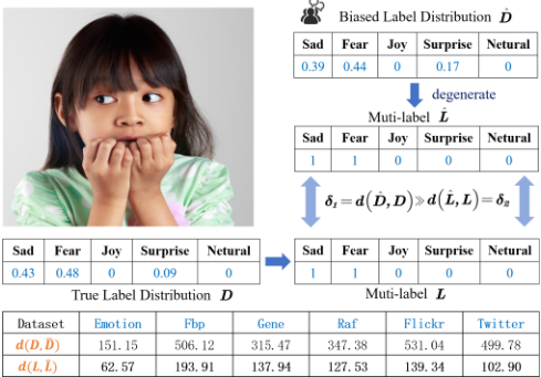
However, recent evidence shows that the label distribution tends to be full-rank [Wang and Geng, 2021], and naive apply of low-rank approximation on biased observation leads to inaccurate recovery and performance degradation. In this paper, we address the LDL with biased annotations problem from a novel perspective, where we first degenerate the soft label distribution into a hard multi-hot label and then recover the true label information for each instance. This idea stems from an insight that assigning hard multi-hot labels is often easier than assigning a soft label distribution, and it shows stronger immunity to noise disturbances, leading to smaller label bias. As shown in Fig. 1, one images from the Real-world Affective Faces (RAF) [Li and Deng, 2019] reveals significant discrepancies between the biased and true soft label distributions ( ˆD and D). However, their corresponding multi-hot label (ˆL and L) exhibit much smaller differences. This phenomenon holds across datasets, as demonstrated by the Tables in Fig. 1. Moreover, while label distributions are inherently full-rank [Wang and Geng, 2021], multi-label spaces are widely regarded as low-rank [Zhu et al., 2017], making them more computationally efficient for correlation modeling. The contributions of this work are summarized as
1 LDL is similar to learning from soft labels, but the soft-label formulation focuses on single-label problems (i.e., there is only one true label for each instance), while LDL considers multi-label problems (i.e., each instance can have multiple true labels).
- We utilize multi-label information and label correlations to model the recovery of the true label distribution and propose the BLDL algorithm (Sections 2).
- Extensive theoretical analysis is provided, including convergence guarantees and generalization error bounds (Section 4).
- The effectiveness of the method is validated through comprehensive experiments, with superior performance demonstrated and insights verified. (Section 5).
1.1 Preliminaries
Denote X ∈ Rd×n as the feature matrix, where d is the feature dimensionality and n is the number of instances. The label space is Y = {y1, . . . , ym}, where m is the number of labels. The accurate training set for LDL is T = {(xi, di)}ni=1 , with di = [dy1 xi , · · · , dym xi ]⊤ ∈ Rm, satisfying dyxi ≥ 0 for all y ∈ Y and ∑y dyxi = 1. The label distribution matrix is D = [d1, . . . , dn] ∈ Rm×n . We assume the observed label distribution ˆD ∈ Rm×n is biased, while the true label distribution is unknown. The goal is to learn a decision function G : Rd×n → Rm×n using the training set {X, ˆD}, such that G(Xi:) ≈ Di:.
2 The BLDL Approach
A common approach in multi-label learning to capture label correlations is leveraging low-rank modeling on the output space. This can be formulated as the following optimization problem:min
where W ∈ Rm×d is the learned weight matrix mapping the feature space to the multi-label space L ∈ Rm×n . The first term captures label correlations via low-rank modeling [Jia et al., 2019].
Annotating label distributions is challenging, often introducing bias. As an extension of MLL, certain bias LDL methods leverage label correlations to recover true distributions from biased ones while learning an effective model. These methods can be formulated as:
where D ∈ Rm×n is the recovered label distribution, E ∈ Rm×n is the annotation bias, and R applies regularization. δ1 and δ2 represent the reconstruction errors in the optimization process.
However, recent evidence shows that the label distribution tends to be full-rank [Wang and Geng, 2021], and naive apply of low-rank approximation on biased observation leads to inaccurate recovery and performance degradation. In this paper, we address the above limitations of existing methods. Our method are enhance as below:
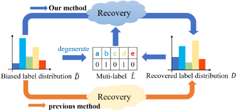
where O ∈ Rm×m models the degradation from label distribution to multi-label, and ˆL ∈ Rm×n represents the multilabel derived from biased distribution. D is recovered label distribution. Parameters α, β, and λi control the term weightings. Our method consists of three parts. The first part is label distribution recovery, where we use both the biased label distribution and its multi-label representation. Recovering the label distribution via the multi-label space is more reliable than relying directly on the biased distribution, as the discrepancy between the biased and true distributions is much larger than between their multi-label representations. By constraining the degradation of the recovered true distribution to the multi-label space (Condition 2), the reliability of the process is ensured. We also require that the difference between the recovered true distribution and the biased distribution be bounded by δ1 (Condition 1) to control the recovery of the label distribution. The second part is label distribution learning, where we impose a low-rank constraint on the multi-label space (instead of the label distribution space, since it is fullrank) to capture label correlations (the first, third, and fourth terms of Eq. (3)). The final part is the multi-label mapping process, where we learn the mapping from multi-labels to label distributions (the second and fifth terms of Eq. (3)). The algorithm flow chart is shown in Fig. 2,
3 Optimization
To solve model (3), we relax the rank by its convex alternative, nuclear norm [Gu et al., 2014], and then apply the ADMM [Boyd et al., 2011] for efficient optimization. The corresponding augmented Lagrangian function is:
where Z is a splitting variable of WXO, Λ is the Lagrange multiplier, and ρ is positive penalty parameter. The optimization is performed by iteratively updating W,O,D,Z,Λ as follows:
1) W-subproblem is formulated as:
To obtain the solution, we set the derivative of the objective with respect toW to zero, and we get:
2) O-subproblem is formulated as:
Similar to the solution for W, and we get:
3) D-subproblem is formulated as:
Similar to the solution above, and we get:
4) Z-subproblem is formulated as:
The solution has closed-form via the soft-thresholding operator [Rajwade et al., 2013]:
5) Finally, update the Lagrange Multipliers
and update ρ by µρ for some µ > 1.
4 Theoretical Analysis
We first analyze the convergence of the above algorithm in solving the proposed BLDL model.
Theorem1. All these iterative solutionsW,O,D,Z,Λgenerated by the above ADMM procedure are bounded and convergent.
We then establish the generalization error bound for the proposed BLDL framework.
Theorem 2. The generalization error of the model, defined as Egen = ED [∥WX - Dtrue∥2F ], which is bounded as follows:
where δ4 is the upper bound imposed by the optimization constraint, δ is the Restricted Isometry Property (RIP) constant, δ3 bounds the deviation between D and ˆD, and O ( rank(WXO) √n ) accounts for the complexity induced by nuclear norm regularization.
According to this theorem, it ensures that the recovered label distribution is robust to noise, consistent with biased observations, and achieves model simplicity via low-rank constraints. All the proof detail can be found in the appendix.
| ID | Data sets | Objects | Features | Labels |
|---|---|---|---|---|
| 1 | Flickr | 6690 | 200 | 8 |
| 2 | 6027 | 200 | 8 | |
| 3 | Emotion6 | 1980 | 12 | 7 |
| 4 | Fbp5500 | 5500 | 512 | 5 |
| 5 | SCUT-FBP | 1500 | 300 | 5 |
| 6 | RAF-ML | 4908 | 200 | 6 |
| 7 | Gene | 17892 | 36 | 68 |
| 8 | Scene | 2000 | 294 | 9 |
| 9 | SBU-3DFE | 2500 | 243 | 6 |
| 10 | SJAFFE | 213 | 243 | 6 |
| 11 | Spo5 | 2465 | 24 | 3 |
| 12 | Spoem | 2465 | 24 | 2 |
5 Experiments
5.1 Datasets
We evaluate our proposed method on 12 real-world datasets. The datasets cover diverse domains: Flickr, Twitter [Yang et al., 2017], and Emotion6 [Peng et al., 2015] describe emotional responses to images. Fbp5500 and SCUT-FBP focus on facial beauty perception [Ren and Geng, 2017]. RAF-ML is a text dataset for sentiment analysis [Li and Deng, 2019]. The Gene dataset analyzes relationships between genes and diseases [Yu et al., 2012]. Scene is derived from a multi-label dataset by converting label rankings into label distributions [Geng and Xia, 2014]. SJAFFE and SBU-3DFE are facial emotion datasets collected from JAFFE [Lyons et al., 1998] and BU-3DFE [Yin et al., 2006], respectively. Finally, Spo5 and Spoem are yeast datasets obtained from biological experiments [Geng, 2016].
5.2 EvaluationMetrics:
We employ six metrics [Kou et al., 2025] to evaluate the performance of all LDL methods: Chebyshev distance (Chebyshev↓), Clark distance (Clark↓), Kullback-Leibler divergence (KL↓), Canberra metric (Canberra↓), intersection similarity (Intersection↑), and cosine coefficient (Cosine↑.
5.3 Biased LDLGeneration:
We simulate biased label distributions by modeling experts' annotations as a voting process, consistent with the Central Limit Theorem. Specifically, Gaussian noise (0, Cm ) is added to the true label distributions, followed by normalization to ensure the distribution constraint holds. Here, m denotes the number of labels, and C controls the deviation degree of the biased label distributions. In our experiments, C is set to 0.1, 0.2, and 0.3 to evaluate varying levels of bias. Parameter C was set to 0.1, 0.2, and 0.3.
5.4 ComparingMethods
We compare our proposed method with seven state-of-the-art LDL methods, briefly introduced as follows:
- DN-ILDL [Kou et al., 2024a]: Handles label-dependent and instance-dependent noise by utilizing linear mappings, group sparsity, and graph regularization.
- LDL-SCL [Zheng et al., 2018]: Explores local sample correlations through the construction of a local correlation vector.
- LDLLC [Jia et al., 2018]: Captures label correlations via a distance-based mapping function.
- LRS-LDL [Kou et al., 2023]: Learns a low-rank linear mapping for ground truth and a sparse mapping for noise.
- LDLLDM [Wang and Geng, 2021]: Models both global and local label correlations by learning the underlying manifold structure of label distributions.
- EDL-LRL [Jia et al., 2019]: Utilizes local label correlations to effectively capture varying intensities of multiple emotions.
- TLRLDL [Kou et al., 2024b]: Integrates an auxiliary multi-label learning process within LDL to capture lowrank label correlations.
The hyperparameters setting. The hyperparameters for all methods were set according to their respective publications. For BLDL, the parameters α, β, γ, λ1, and λ2 were fine-tuned over the range {0.1, 0.05, 0.01, 0.005, 0.001}. The parameter η was selected from {1, 10, 50, 100, 150}, and T was fixed at 0.5. Each method was evaluated using ten-fold cross-validation to ensure robustness.
5.5 Results and Discussion
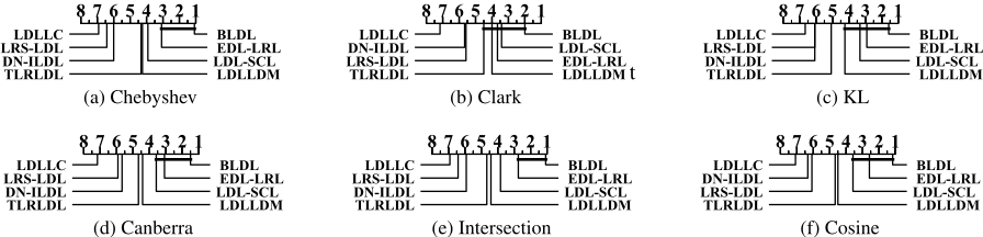
Table 2 shows the experimental results (mean±std) of various methods on eight datasets for Clark and Cosine metrics. For C = 0.1, the Friedman test [Demˇsar, 2006] rejected the null hypothesis that "all methods perform equally" (Table 3). Subsequently, the Bonferroni-Dunn test [Demˇsar, 2006] was used to compare BLDL with others, where methods differing by more than one Critical Difference (CD) are considered significantly different. CD diagrams in Fig. 3 highlight methods within one CD of BLDL connected by a thin line, confirming BLDL's significant advantage. From these results, we conclude:
- Top-1 dominance. BLDL achieves top-1 performance in 85.42% (41/48) of all configurations and consistently ranks first across all metrics by effectively addressing bias in the learning process.
- Benefit of joint modeling. Compared to methods focusing solely on label correlations (e.g., LDLLC, LDLLDM), BLDL performs better since those methods ignore the bias present in label distributions.
- Superiority over bias-only approaches. BLDL also outperforms methods that address bias alone (e.g., DNILDL, LRS-LDL) by additionally leveraging label correlations-an exploit these bias-only methods fail to capture effectively.
5.6 Ablation Study
To validate the proposed method, we design two ablated versions: (i) BLDL-a: Removes the multi-label recovery process (i.e. drops the first term in Eq. (3)). (ii)BLDL-b: Replaces the low-rank constraint onWXOwith one onWO, thus applying low-rank modeling in the label-distribution space instead of the multi-label feature space.
| C | Metric | BLDL | DN-ILDL | LDL-SCL | LDLLC | LRS-LDL | LDLDM | EDL-LDL | TLRLDL | |
|---|---|---|---|---|---|---|---|---|---|---|
| Fli | 0.1 | Clark 2.1146±.0020 Cosine 0.8368±.0003 | 2.1990±.0008 0.5516±.0002 | 2.1576±.0001 0.7356±.0001 | 2.1990±.0042 0.5781±.0038 | 2.2029±.0028 0.5537±.0005 | 2.1705±.0001 0.6964±.0001 | 2.1797±.0001 0.7436±.0001 | 2.1777±.0005 0.6421±.0009 | |
| 0.2 | Clark 2.1175±.0010 Cosine 0.8316±.0034 | 2.1969±.0153 0.5531±.0052 | 2.1587±.0001 0.7289±.0001 | 2.1984±.0021 0.5781±.0004 | 2.1984±.0078 0.5556±.0027 | 2.1707±.0001 0.6869±.0001 | 2.1758±.0001 0.7414±.0001 | 2.1768±.0020 0.6356±.0006 | ||
| 0.3 | Clark Cosine | 2.1382±.0010 0.8276±.0021 | 2.2018±.0033 0.5510±.0017 | 2.1597±.0001 0.7228±.0001 | 2.1990±.0019 0.5761±.0008 | 2.1985±.0028 0.5554±.0001 | 2.1713±.0001 0.6792±.0001 | 2.1733±.0001 0.7394±.0001 | 2.1778±.0005 0.6322±.0014 | |
| 0.1 | Clark Cosine | 2.2517±.0028 0.8582±.0025 | 2.4072±.0037 0.4955±.0013 | 2.3602±.0001 0.7537±.0001 | 2.3957±.0039 0.5617±.0022 | 2.4043±.0040 0.5000±.0008 | 2.3656±.0001 0.7519±.0001 | 2.3874±.0001 0.8134±.0001 | 2.3726±.0001 0.6283±.0004 | |
| Twi 0.2 | Clark Cosine | 2.2783±.0113 0.8535±.0015 | 2.4014±.0008 0.4980±.0009 | 2.3608±.0001 0.7509±.0001 | 2.3897±.0036 0.5621±.0043 | 2.4015±.0020 0.5016±.0017 | 2.3651±.0001 0.7372±.0001 | 2.3827±.0001 0.8124±.0001 | 2.3763±.0069 0.6211±.0037 | |
| 0.3 | Clark Cosine | 2.3051±.0080 0.8480±.0012 | 2.4043±.0050 0.4957±.0018 | 2.3616±.0001 0.7447±.0001 | 2.3906±.0034 0.5575±.0029 | 2.4016±.0020 0.5014±.0016 | 2.3657±.0001 0.7274±.0001 | 2.3790±.0001 0.8106±.0001 | 2.3780±.0017 0.6131±.0003 | |
| 0.1 | Clark Cosine | 1.6237±.0067 0.7462±.0099 | 1.6753±.0032 0.6592±.0008 | 1.6457±.0001 0.7266±.0001 | 1.6875±.0077 0.6700±.0005 | 1.6820±.0113 0.6560±.0047 | 1.6404±.0002 0.7417±.0001 | 1.6423±.0001 0.7639±.0001 | 1.6697±.0114 0.6841±.0020 | |
| Emo 0.2 | Clark Cosine | 1.6408±.0008 0.7499±.0004 | 1.6716±.0174 0.6613±.0042 | 1.6480±.0001 0.7227±.0001 | 1.6840±.0106 0.6701±.0063 | 1.6774±.0031 0.6565±.0005 | 1.6432±.0002 0.7370±.0001 | 1.6412±.0002 0.7589±.0001 | 1.6677±.0020 0.6816±.0009 | |
| 0.3 | Clark Cosine | 1.6295±.0004 0.7458±.0030 | 1.6753±.0051 0.6579±.0004 | 1.6491±.0001 0.7193±.0001 | 1.6848±.0104 0.6685±.0059 | 1.6775±.0031 0.6564±.0005 | 1.6467±.0001 0.7304±.0001 | 1.6402±.0002 0.7574±.0001 | 1.6799±.0001 0.6771±.0014 | |
| 0.1 | Clark Cosine | 1.2494±.0047 0.9342±.0010 | 1.5052±.0013 0.6571±.0005 | 1.4032±.0001 0.8596±.0001 | 1.4866±.0010 0.6772±.0035 | 1.5039±.0041 0.6617±.0014 | 1.4391±.0001 0.7929±.0001 | 1.3360±.0001 0.9169±.0001 | 1.6697±.0021 0.6841±.0004 | |
| Fbp 0.2 0.3 | Clark Cosine Clark | 1.2974±.0024 0.9264±.0012 | 1.5054±.0021 0.6571±.0003 | 1.4115±.0001 0.8478±.0001 | 1.4891±.0001 0.6754±.0026 1.4895±.0003 | 1.5027±.0003 0.6625±.0009 1.5028±.0003 | 1.4475±.0001 0.7795±.0001 1.4530±.0001 | 1.3472±.0001 0.9127±.0001 1.3542±.0001 | 1.4579±.0015 0.7619±.0027 1.4623±.0004 | |
| 0.1 | Cosine | 1.3084±.0053 0.9251±.0007 | 1.5040±.0009 0.6577±.0004 | 1.4182±.0001 0.8367±.0001 | 0.6747±.0022 1.4838±.0056 | 0.6622±.0009 1.4985±.0031 | 0.7695±.0001 1.4265±.0001 0.8089±.0001 | 0.9083±.0001 1.3908±.0001 0.8405±.0001 | 0.7553±.0005 1.4735±.0036 0.7217±.0028 | |
| Scu | Clark Cosine Clark 1.3936±.0090 Cosine 0.8344±.0013 | 1.3869±.0051 0.8409±.0075 | 1.4955±.0044 0.6647±.0016 1.4930±.0037 0.6653±.0013 | 1.4494±.0001 0.7775±.0001 1.4540±.0001 0.7761±.0001 | 0.6717±.0068 1.4796±.0055 0.6687±.0056 | 0.6672±.0008 1.4999±.0003 0.6665±.0018 | 1.4357±.0001 0.7965±.0001 | 1.3965±.0001 0.8369±.0001 1.4022±.0001 0.834±.0001 | 1.4723±.0045 0.7213±.0010 | |
| 0.2 0.3 | Clark 1.3934±.0066 Cosine Clark | 0.8341±.0032 1.3864±.0003 | 1.4971±.0049 0.6634±.0013 1.6119±.0037 | 1.4562±.0001 0.7683±.0001 1.5534±.0001 0.7433±.0001 | 1.4807±.0048 0.6669±.0069 1.6115±.0027 0.6360±.0011 | 1.5001±.0005 0.6662±.0019 1.6102±.0012 0.6455±.0001 | 1.4394±.0001 0.7908±.0001 1.6025±.0001 0.6541±.0001 | 1.5410±.0001 0.7580±.0001 | 1.4748±.0005 0.7131±.0025 1.5688±.0031 | |
| Raf 0.1 | Cosine 0.8734±.0006 | 1.4205±.0050 | 0.6413±.0006 1.6082±.0005 | 1.5586±.0001 | 1.6071±.0021 | 1.6043±.0034 | 1.6015±.0001 | 1.5464±.0001 | 0.7200±.0011 | |
| 0.2 | Clark Cosine | 0.8630±.0007 | 0.6418±.0006 | 1.5638±.0001 | 0.6356±.0031 | 0.6472±.0018 | 0.6566±.0001 | 0.7506±.0001 | 1.5723±.0052 0.7153±.0016 | |
| 0.3 | Clark 1.4270±.0019 Cosine 0.8519±.0010 | 1.6098±.0005 0.6417±.0001 | 0.7349±.0001 0.7260±.0001 | 1.6076±.0019 0.6352±.0029 | 1.6044±.0033 0.6469±.0018 | 1.6034±.0001 0.6532±.0001 | 1.5496±.0001 0.7469±.0001 | 1.5711±.0001 0.7103±.0022 | ||
| 0.1 | Clark Cosine | 2.1149±.0179 0.8353±.0023 | 2.1151±.0006 0.8342±.0003 | 2.1230±.0001 0.8337±.0001 | 2.1618±.0087 0.8196±.0006 | 2.1222±.0069 0.8342±.0009 | 2.1248±.0001 0.8338±.0001 | 2.1240±.0003 0.8339±.0001 | 2.1312±.0030 0.8317±.0005 | |
| Gen | Clark | 2.1228±.0107 | 2.1246±.0066 | 2.1591±.0018 | 2.1256±.0222 | 2.1245±.0001 | 2.1236±.0001 | |||
| 0.2 | Cosine Clark 2.1225±.0035 | 0.8340±.0016 | 0.8336±.0021 2.1269±.0035 | 2.1237±.0001 0.8333±.0001 2.1225±.0005 | 0.8202±.0014 2.1591±.0018 | 0.8334±.0028 2.1256±.0222 | 0.8337±.0001 2.1249±.0006 | 0.8338±.0001 2.1240±.0005 | 2.1312±.0127 0.8329±.0016 2.1296±.0187 | |
| 0.3 0.1 | Cosine 0.8338±.0003 Clark Cosine | 2.4900±.0012 0.7037±.0045 | 0.8335±.0007 2.4848±.0017 0.5748±.0003 | 0.8333±.0001 2.4654±.0001 0.6770±.0001 | 0.8202±.0014 2.4915±.0019 0.5572±.0008 | 0.8334±.0028 2.4747±.0012 0.5806±.0013 | 0.8336±.0001 2.4702±.0001 0.6431±.0001 | 0.8337±.0001 2.4775±.0001 0.6500±.0001 | 0.8334±.0012 2.4736±.0001 0.6253±.0007 | |
| Sce 0.2 | Clark Cosine | 2.4808±.0129 0.7010±.0010 | 2.4829±.0001 0.5753±.0007 | 2.4668±.0001 0.6692±.0001 | 2.4950±.0066 0.5553±.0018 | 2.4819±.0059 0.5780±.0029 | 2.4711±.0001 0.6367±.0001 | 2.4751±.0001 0.6469±.0001 | 2.4771±.0040 0.6205±.0034 | |
| 0.3 | Clark Cosine | 2.5100±.0123 0.6876±.0026 | 2.4859±.0057 0.5738±.0034 | 2.4683±.0001 0.6611±.0001 | 2.4951±.0066 0.5551±.0016 | 2.4820±.0059 0.5779±.0030 | 2.4721±.0002 0.6328±.0001 | 2.4758±.0001 0.6455±.0001 | 2.4799±.0040 0.6168±.0029 | |
| top-1 times | 41 | 0 | 3 | 0 | 0 | 0 | 4 | 0 | ||
| Critical Value (α = 0.05) | Evaluation metric | Cheb | Clark | KL | Canber | Intersec | Cosine |
| 2.1310 | Friedman Statistics FF | 17.6522 | 8.2619 | 12.6744 | 12.5264 | 19.2706 | 22.4616 |

| BLDL vs. | Chebyshev | Clark | KL | Canberra | Intersection | Cosine |
|---|---|---|---|---|---|---|
| BLDL-a | win[4.88e-04] | win[3.42e-03] | win [4.88e-04] | win[4.88e-04] | win[4.88e-04] | win[4.88e-04] |
| BLDL-b | win[9.77e-04] | win [9.28e-03] | win[5.37e-03] | win[4.88e-04] | win [9.77e-04] | win[4.88e-04] |
We compare BLDL-a and BLDL-b with the full BLDL using biased label distributions generated with C = 0.1. Fig. 4 shows results on seven datasets for Chebyshev and Intersection metrics. Wilcoxon signed-rank tests [Demˇsar, 2006] confirm the statistical significance of BLDL over both ablated versions (Table 4). From these experiments, we draw three key observations:
- Importance of multi-label recovery. Comparing BLDL-a vs. BLDL reveals a significant performance drop when the multi-label recovery step is removed, underscoring the critical role of leveraging multiple pseudo-labels to denoise and recover true distributions.
- Effect of low-rank constraint location. Comparing BLDL-b vs. BLDL shows that enforcing low-rank structure on WXO (the recovered multi-label space) outperforms constrainingWO alone, since the multi-label embedding X is intrinsically low-rank and more robust to annotation noise.
- Combined benefits. The full BLDL, which both recovers multi-label distributions and constrains the low-rank structure in the correct space, consistently achieves the best results across all metrics and datasets.
5.7 Validation of Hypothesis
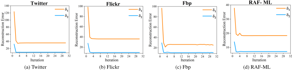
We computed the difference between the recovered label distribution and the biased label distribution during the training phase, denoted as δ1, and the difference between the multilabel corresponding to the recovered label distribution and the multi-label corresponding to the biased distribution, denoted as δ2. As show in Fig. 5, it can be observed that δ1 is consistently greater than δ2 until convergence. Therefore, during the label distribution recovery phase, multi-label information is more reliable than the biased label distribution information.
5.8 Analysis of Label Distribution Recovery
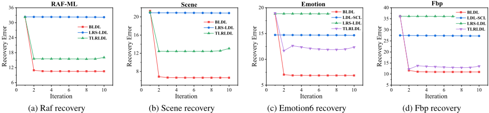
We evaluate the recovery error of label distributions during training using the Frobenius norm ∥Drecover - Dtruth∥F , as shown in Fig. 6. Our method achieves lower recovery error compared to LRS-LDL, demonstrating the benefit of leveraging multi-label information. Additionally, it outperforms TLRLDL by addressing biases in the learning process, further improving recovery accuracy.
5.9 Parameter Sensitivity Analysis
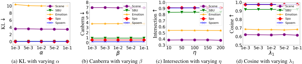
We analyze the sensitivity of α, β, η, λ1, with α, β, λ1 chosen from {0.1, 0.05, 0.01, 0.005, 0.001} and η from {1, 10, 50, 100, 150}. Experiments on five datasets (Scene, SBU, Emotion, Spo, Spoem) show in Fig. 7 that BLDL exhibits stable performance, demonstrating robustness to parameter variations.
6 Conclusion
This paper introduces a novel framework, Biased Label Distribution Learning (BLDL), to address label distribution learning under biased annotations. Unlike conventional methods, BLDL first converts biased soft label distributions into multi-label representations, effectively mitigating annotation noise and bias. It further exploits the intrinsic low-rank structure of multi-label spaces to reliably recover true label distributions. Comprehensive theoretical analysis and experiments on diverse real-world datasets demonstrate that BLDL significantly enhances the accuracy and robustness of label distribution recovery, outperforming state-of-the-art methods.
Acknowledgments
This work was supported in part by the Jiangsu Science Foundation (BK20243012, BG2024036, BK20230832), the JST ASPIRE Program (JPMJAP2405), the National Natural Science Foundation of China (62125602, U24A20324, 92464301, 62306073), the China Postdoctoral Science Foundation (2022M720028), the Xplorer Prize, and the National Natural Science Foundation of China under Grant U24A20322. Additional support was provided by the Big Data Computing Center of Southeast University. Zhiqiang Kou and Hailin Wang conducted this work during their visit to the RIKEN Center for Advanced Intelligence Project, Japan.
Zhiqiang Kou, Si Qin, and Hailin Wang contributed equally to this work. Yuheng Jia and Xin Geng are the corresponding authors.
@inproceedings{ijcai2025p617,
  title     = {Label Distribution Learning with Biased Annotations Assisted by Multi-Label Learning},
  author    = {Kou, Zhiqiang and Qin, Si and Wang, Hailin and Wang, Jing and Xie, Mingkun and Chen, Shuo and Jia, Yuheng and Liu, Tongliang and Sugiyama, Masashi and Geng, Xin},
  booktitle = {Proceedings of the Thirty-Fourth International Joint Conference on
               Artificial Intelligence, {IJCAI-25}},
  publisher = {International Joint Conferences on Artificial Intelligence Organization},
  editor    = {James Kwok},
  pages     = {5545--5553},
  year      = {2025},
  month     = {8},
  note      = {Main Track},
  doi       = {10.24963/ijcai.2025/617},
  url       = {https://doi.org/10.24963/ijcai.2025/617},
}
TY - CPAPER TI - Label Distribution Learning with Biased Annotations Assisted by Multi-Label Learning AU - Kou, Zhiqiang AU - Qin, Si AU - Wang, Hailin AU - Wang, Jing AU - Xie, Mingkun AU - Chen, Shuo AU - Jia, Yuheng AU - Liu, Tongliang AU - Sugiyama, Masashi AU - Geng, Xin T2 - Proceedings of the Thirty-Fourth International Joint Conference on Artificial Intelligence, IJCAI-25 PB - International Joint Conferences on Artificial Intelligence Organization PY - 2025 SP - 5545 EP - 5553 DO - 10.24963/ijcai.2025/617 UR - https://doi.org/10.24963/ijcai.2025/617 ER -Copied
Machine-readable versions of this paper, for tools and AI agents:





