
Linear Trading Position with Sparse Spectrum
Proceedings of the Thirty-Fourth International Joint Conference on Artificial Intelligence. Main Track. Pages 5554-5562.
https://doi.org/10.24963/ijcai.2025/618
Keywords
- Constraint Satisfaction and Optimization: CSO: Solvers and tools
- Machine Learning: ML: Optimization
- Multidisciplinary Topics and Applications: MTA: Finance
Abstract
The principal portfolio approach is an emerging method in signal-based trading. However, these principal portfolios may not be diversified to explore the key features of the prediction matrix or robust to different situations. To address this problem, we propose a novel linear trading position with sparse spectrum that can explore a larger spectral region of the prediction matrix. We also develop a Krasnosel'skii-Mann fixed-point algorithm to optimize this trading position, which possesses the descent property and achieves a linear convergence rate in the objective value. This is a new theoretical result for this type of algorithms. Extensive experiments show that the proposed method achieves good and robust performance in various situations.
- [Bauschke and Combettes, 2017] Heinz H. Bauschke and Patrick L. Combettes. Convex Analysis and Monotone Op- erator Theory in Hilbert Space. Springer, New York, 2nd edition, 2017.
- [Bot ¸and Nguyen, 2023] Radu Bot ¸and Dang-Khoa Nguyen. Fast krasnosel'skiȋ-mann algorithm with a convergence rate of the fixed point iteration of o 1 k . SIAM Journal on Numerical Analysis, 61:2813-2843, 11 2023.
- [Bruni et al., 2016] Renato Bruni, Francesco Cesarone, An- drea Scozzari, and Fabio Tardella. Real-world datasets for portfolio selection and solutions of some stochastic domi- nance portfolio models. Data in Brief, 8:858-862, 2016.
- [Cai et al., 2010] Jian-Feng Cai, Emmanuel J. Candès, and Zuowei Shen. A singular value thresholding algorithm for matrix completion. SIAM Journal on Optimization, 20(4):1956-1982, 2010.
- [Candès and Recht, 2012] Emmanuel Candès and Benjamin Recht. Exact matrix completion via convex optimization. Communications of the ACM, 55(6):111-119, Jun. 2012.
- [Collin-Dufresne et al., 2020] Pierre Collin-Dufresne, Kent Daniel, and Mehmet Saglam. Liquidity regimes and op- timal dynamic asset allocation. Journal of Financial Eco- nomics, 136(2):379-406, 2020.
- [Cui et al., 2020] Shuhao Cui, Shuhui Wang, Junbao Zhuo, Liang Li, Qingming Huang, and Qi Tian. Towards dis- criminability and diversity: Batch nuclear-norm maxi- mization under label insufficient situations. In Proceed- ings of the IEEE/CVF Conference on Computer Vision and Pattern Recognition (CVPR), June 2020.
- [Fama and French, 2015] Eugene F. Fama and Kenneth R. French. A five-factor asset pricing model. Journal of Fi- nancial Economics, 116(1):1-22, 2015.
- [Gârleanu and Pedersen, 2013] Nicolae Gârleanu and Lasse Heje Pedersen. Dynamic trading with predictable returns and transaction costs. The Journal of Finance, 68(6):2309-2340, 2013.
- [Gibbons et al., 1989] Michael R. Gibbons, Stephen A. Ross, and Jay Shanken. A test of the efficiency of a given portfolio. Econometrica, 57(5):1121-1152, 1989.
- [Gupta and Kelly, 2019] Tarun Gupta and Bryan Kelly. Fac- tor momentum everywhere. The Journal of Portfolio Man- agement, 45(45):13-36, 2019.
- [Kelly et al., 2019] Bryan T. Kelly, Seth Pruitt, and Yinan Su. Characteristics are covariances: A unified model of risk and return. Journal of Financial Economics, 134(3):501-524, 2019.
- [Kelly et al., 2023a] Bryan Kelly, Semyon Malamud, and Lasse Heje Pedersen. Principal portfolios. The Journal of Finance, 78(1):347-387, 2023.
- [Kelly et al., 2023b] Bryan Kelly, Diogo Palhares, and Seth Pruitt. Modeling corporate bond returns. The Journal of Finance, 78(4):1967-2008, 2023.
- [Krasnosel'skiȋ, 1955] Mark Aleksandrovich Krasnosel'skiȋ. Two remarks on the method of successive approximations. Uspekhi Mat. Nauk, 10(1):123-127, 1955.
- [Lacroix et al., 2018] Timothee Lacroix, Nicolas Usunier, and Guillaume Obozinski. Canonical tensor decomposi- tion for knowledge base completion. In Jennifer Dy and Andreas Krause, editors, Proceedings of the 35th Inter- national Conference on Machine Learning, volume 80 of Proceedings of Machine Learning Research, pages 2863- 2872. PMLR, 10-15 Jul 2018.
- [Lai and Yang, 2023] Zhao-Rong Lai and Haisheng Yang. A survey on gaps between mean-variance approach and ex- ponential growth rate approach for portfolio optimization. ACM Computing Surveys, 55(2):1-36, Mar. 2023. Article No. 25.
- [Lai et al., 2018] Zhao-Rong Lai, Pei-Yi Yang, Liangda Fang, and Xiaotian Wu. Short-term sparse portfolio op- timization based on alternating direction method of multi- pliers. Journal of Machine Learning Research, 19(63):1- 28, Oct. 2018.
- [Lai et al., 2020] Zhao-Rong Lai, Liming Tan, Xiaotian Wu, and Liangda Fang. Loss control with rank-one covariance estimate for short-term portfolio optimization. Journal of Machine Learning Research, 21(97):1-37, Jun. 2020.
- [Lai et al., 2024] Zhao-Rong Lai, Xiaotian Wu, Liangda Fang, and Ziliang Chen. A de-singularity subgradient approach for the extended weber location problem. In Proceedings of the Thirty-Third International Joint Con- ference on Artificial Intelligence, IJCAI-24, pages 4370- 4379. International Joint Conferences on Artificial Intelli- gence Organization, 8 2024. Main Track. IJCAI
- [Li et al., 2016] Bin Li, Doyen Sahoo, and Steven C.H. Hoi. OLPS: a toolbox for on-line portfolio selection. Journal of Machine Learning Research, 17(1):1242-1246, 2016.
- [Lin et al., 2024a] Yizun Lin, Zhao-Rong Lai, and Cheng Li. A globally optimal portfolio for m-sparse sharpe ra- tio maximization. In Advances in Neural Information Pro- cessing Systems, volume 37, pages 17133-17160, 2024.
- [Lin et al., 2024b] Yizun Lin, Yangyu Zhang, Zhao-Rong Lai, and Cheng Li. Autonomous sparse mean-CVaR portfolio optimization. In Proceedings of the 41st Inter- national Conference on Machine Learning, volume 235 of Proceedings of Machine Learning Research, pages 30440-30456. PMLR, 21-27 Jul 2024.
- [Lintner, 1965] John Lintner. The valuation of risk assets and the selection of risky investments in stock portfolios and capital budgets. Review of Economics and Statistics, 47(1):13-37, Feb. 1965.
- [Magdon-Ismail and Atiya, 2004] Malik Magdon-Ismail and Amir F. Atiya. Maximum drawdown. Risk Magazine, 10:99-102, 2004.
- [Mann, 1953] W. Robert Mann. Mean value methods in iter- ation. Proceedings of the American Mathematical Society, 4:506-510, 1953.
- [Moreau, 1965] Jean-Jacques Moreau. Proximité et dualité dans un espace hilbertien. Bull. Soc. Math. France, 93(2):273-299, 1965.
- [Moskowitz et al., 2012] Tobias J. Moskowitz, Yao Hua Ooi, and Lasse Heje Pedersen. Time series momentum. Journal of Financial Economics, 104(2):228-250, 2012.
- [Rockafellar and Wets, 2009] R Tyrrell Rockafellar and Roger J-B Wets. Variational Analysis, volume 317. Springer Science & Business Media, 2009.
- [Sharpe, 1966] William F. Sharpe. Mutual fund perfor- mance. Journal of Business, 39(1):119-138, Jan. 1966.
- [Treynor and Black, 1973] Jack L. Treynor and Fischer Black. How to use security analysis to improve portfolio selection. Journal of Business, 46(1):66-86, Jan. 1973.
- [You et al., 2020] Jiaxuan You, Xiaobai Ma, Yi Ding, Mykel J Kochenderfer, and Jure Leskovec. Handling missing data with graph representation learning. In H. Larochelle, M. Ranzato, R. Hadsell, M.F. Balcan, and H. Lin, editors, Advances in Neural Information Process- ing Systems, volume 33, pages 19075-19087.
References were extracted automatically from the PDF and may contain errors.
Full text extracted automatically from the PDF; figures, tables and equations may differ. The PDF is the version of record.
1 Introduction
In general, asset pricing starts with finding some current signals St ∈ RN as proxies for the conditional expected returns Rt+1 ∈ RN at the next time, which gives rise to signal-based trading [Gibbons et al., 1989]. Since asset correlation exists in most cases, linear trading strategies are proposed to exploit cross-predictability (see Figure 1) [Gˆarleanu and Pedersen, 2013; Collin-Dufresne et al., 2020; Lai et al., 2024; Lin et al., 2024b; Lin et al., 2024a]. Recently, [Kelly et al., 2023a] propose to directly combine signals and returns into a bi-linear form with a "prediction matrix", and extract several principal portfolios (PP) of this prediction matrix to form a linear trading position (LTP). [Kelly et al., 2023b] further propose a conditional factor model for individual corporate bond based on instrumented principal components analysis (IPCA,[Kelly et al., 2019]). This approach exploits the predictability from both own-asset signal and other-asset signals, while keeping a closed-form LTP. It not only keeps a concise portfolio but also improves interpretability of LTP in finance, which leads a new direction in future research.
However, LTP composed by several PPs may not be diversified to explore the key features of the prediction matrix.
∗Corresponding author.
** The supplementary material and code for this paper are available at https://github.com/laizhr/LTPSS.
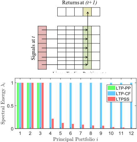
First, it is recognized in [Kelly et al., 2023a] that including more PPs into the LTP does not necessarily lead to better performance. Second, the spectral energy of each PP is either 1 (selected) or 0 (non-selected), and cannot be adjusted in the current framework (green or blue bars in Figure 1). Third, the choice of PPs relies on empirical experience. [Kelly et al., 2023a] suggest empirically using the first three PPs (green bars in Figure 1) as they possess the most proportion of singular value magnitude, but it may not be robust to different situations (see Supplementary A.5).
Importance of diversification: given a simple economic system with 10 states and 10 assets. On each trading period, only one state can occur, and each state occurs with 10% probability. If state i occurs, the price of Asset i will increase by 10%, while those of others will decrease by 1%. Then if an investor invests all his/her wealth in only one asset, he/she will have only 10% probability to gain 10% return, but 90% probability to lose 1%. However, if he/she diversifies the wealth equally in 10 assets (each with 10% of the position), he/she will have 100% probability to gain 1% return without taking the risk of losing wealth.
The same law also holds for PPs, where each PP can be considered as an asset in the above example. Then the diversification over PPs leads to the sparse spectrum concept that has been widely used in various machine learning scenarios, such as matrix completion [Cai et al., 2010; Cand`es and Recht, 2012], knowledge base completion [Lacroix et al., 2018], graph representation learning [You et al., 2020], and insufficient-label recognition [Cui et al., 2020]. We aim to employ this concept in the LTP framework to extract the key features of the prediction matrix (red bars in Figure 1). There are some main difficulties: 1. This problem has a three-part complicated non-differentiable geometrical structure with the Frobenius, nuclear, and spectral norms. A common solver is the semi-definite programming (SDP) with a conic reformulation, which is a surrogate model that cannot achieve fullreinvestment and thus result in poor performance. 2. The projection onto the self-financing constraint [Lai et al., 2020; Lai and Yang, 2023] is nonlinear and non-orthogonal, which rules out most projected subgradient approaches that require orthogonality and the inner product property of the Hilbert space. 3. The descent property and the convergence rate of the solving algorithm are difficult to established.
To address the above challenges, we mainly offer the following contributions. 1. We propose a Linear Trading Position with Sparse Spectrum (LTPSS) that can explore a larger spectral region of the observation matrix, while keeping a sparse and concise representation. 2. We prove that the nonlinear and non-orthogonal projection onto the feasible set is non-expansive, which is crucial to the convergence of the whole solving algorithm. 3. We develop a Krasnosel'ski˘ıMann (KM) fixed-point algorithm to solve LTPSS. It possesses the descent property and achieves a linear convergence rate in the objective value. To the best of our knowledge, this is a new theoretical result for KM algorithms, as the current best result is o ( 1k ) in the fixed point iteration gap [Bot¸ and Nguyen, 2023], but not in the objective value. This new finding may reveal greater breakthroughs for KM algorithms.
2 Preliminaries and RelatedWorks
2.1 Linear Trading Position with Principal Portfolios
We start with introducing the concepts of LTP and PP. Let St ∈ RN and Rt+1 ∈ RN be the signals at time t and returns at time (t + 1) for the N assets in a financial market, respectively. The portfolio optimization task is to find an LTP L ∈ RN×N such thatmaxE[S⊤ t LRt+1]. (1)
In finance, a self-financing constraint is usually imposed to ensure a realistic and feasible trading position, which means that no external money can be added to the position once the trading strategy starts [Lai et al., 2020; Lai and Yang, 2023]. In the framework of [Kelly et al., 2023a; Kelly et al., 2023b], the following self-financing constraint is used
where ∥·∥2 denotes the ℓ2 norm (spectral norm) of a matrix. A trivial strategy satisfying this constraint is the simple factor:
where I(N) denotes the identity matrix of N dimensions. It only uses the own signal of each asset to determine its position. The original LTP model can be formulated as:
where tr(·) denotes the trace operator of a matrix. This formulation exploits the commutative law and the linearity of the trace operator:
Π is called a prediction matrix, which contains all the information that can be exploited to determine L. [Kelly et al., 2023a] propose to estimate it by the empirical estimator:
Since the matrix ℓ2 norm is equivalent to the Schatten ∞- norm, it follows from the H¨older's inequality that
where ∥ · ∥∗ denotes the nuclear norm of the matrix. The equality holds if and only if L is linear to ( ˆΠ⊤ ˆΠ)- 1 2 ˆΠ⊤. Since ∥L∥2 ⩽ 1,
is exactly the closed-form solution to (LTP) with the empirical estimator ˆΠ.
Instead of ˆLCF , [Kelly et al., 2023a] propose to use the PPs of ˆΠ to develop the LTP L. To do this, the first step is to conduct the singular value decomposition (SVD) of ˆΠ⊤ as
where U, V ,U ⊤, V ⊤ are orthonormal bases of RN×N . Then the principal components {unv⊤ n }Nn=1 are defined as the PPs of the prediction matrix ˆΠ, where un and vn are the n-th columns of the matrices U and V , respectively. [Kelly et al., 2023a] propose to use the first several PPs to construct an LTP:
where l denotes the number of selected PPs. This LTP has a simple form, and is highly interpretable in the literature of finance. However, it may not be diversified to capture the key features of ˆΠ. First, the setting of l relies on empirical experience. As indicated by [Kelly et al., 2023a], a larger l does not necessarily lead to better results. Second, (LTP-PP) indicates that the spectral energy of a selected PP is fixed as 1, which may not be adaptive to different situations.
2.2 Surrogate Model
There are some surrogate models for the proposed (LTPSS) model in Section 3.1. One main approach is to reformulate (LTPSS) as a semi-definite conic programming 1 (SDCP). Specifically,
where U, V , and l are auxiliary arguments that need to be optimized simultaneously with L. Then the surrogate model of (LTPSS) is:
This model is not equivalent to (LTPSS). It directly replaces ∥L∥∗ in (LTPSS) by l, which is only an upper bound of ∥L∥∗. Besides, the mainstream solvers for (SDCP) are based on interior-point primal-dual algorithms, which cannot achieve the equality ∥L∥2 = 1 but only satisfy ∥L∥2 < 1. In the experiments, we observe that ∥L∥2 ≈ 0.9826 in all the cases, with both absolute solution tolerance and constraint tolerance being 1e - 6. In this case, the investing capital can not be fully exploited and the investing performance is unsatisfactory (see Table 1). Worse still, it significantly increases computational complexity due to the auxiliary arguments U, V , and l. The dimensionality for the constraints of (SDCP) quadruples that of (LTPSS).
3 Methodology
To address the above problems, we propose to expand the spectral region of LTP. First, we consider all the PPs to construct the LTP. Second, we allow for flexible spectral energies in [0, 1]. Third, we impose sparse spectrum on the LTP to extract the key features of the prediction matrix ˆΠ. Fourth, we develop a KM fixed-point algorithm to directly solve (LTPSS) instead of using the defective and deficient surrogate model (SDCP).
3.1 Linear Trading Position with Sparse Spectrum
Since an LTP L ∈ RN×N , our framework is developed on the linear space RN×N , which is more complicated than RN . First of all, we consider RN×N as a Hilbert space, then the trace operator tr(A⊤B) =: ⟨A,B⟩ is the inner product of A and B, for any A,B ∈ RN×N . Moreover, √tr(A⊤A) = ∥A∥F and thus the Frobenius norm is the induced norm from the trace operator for RN×N . First, we give some properties of the constraint set Ω defined in (2).
Proposition 1. Ω is a convex, closed, and bounded subset of RN×N .
1 https://www.seas.ucla.edu/∼vandenbe/236C/lectures/conic.pdf
Hence ∥θA + (1 - θ)B∥2 ∈ Ω and Ω is convex. Since Ω is a sub-level-set of the continuous function ∥ · ∥2, it is closed [Rockafellar and Wets, 2009]. ∥L∥F = √∑Ni=1 λ2i , where {λi}Ni=1 are the singular values of L (singular values are non-negative). (2) indicates that (max1⩽i⩽N λi) ⩽ 1. Hence ∥L∥F ⩽ √N for any L ∈ Ω, which proves that Ω is bounded.
Next, we propose the following LTPSS model:
where η ⩾ 0 is a regularization parameter. f(L) has the gradient ∇f(L) = - ˆΠ⊤, while g(L) is non-differentiable. Furthermore, the constraint L ∈ Ω is also a non-differentiable structure. In summary, (LTPSS) has three parts with the Frobenius, nuclear, and spectral norms, where the latter two are non-differentiable. By dropping either g(L) or L ∈ Ω, it can be reduced to a common problem that can be solved by either projected gradient or proximal gradient methods, respectively. However, with both nondifferentiable parts present, (LTPSS) cannot be effectively and efficiently solved via common approaches.
Fact: there exists at least one solution to (LTPSS). Since F(L) is a continuous function on L and Ω is a convex and compact set, this fact follows from the Weierstrass extreme value theorem.
3.2 Krasnosel'ski˘ı-Mann Fixed-point Algorithm
To address the above difficulty, we develop a KM fixed-point scheme to solve (LTPSS), which alternately minimizes F (L) and projects L onto Ω. Denote the k-th iterate of L by L(k) . Then in the next iteration, we can use a quadratic approximation to F(L):
where β > 0 is the step size parameter (which can be seen later). By ignoring the constant terms with respect to (w.r.t.) the argument L and temporarily relaxing the constraint L ∈ Ω, we minimize Q(L, L(k) ):
which is the proximal mapping of (L(k) + β ˆΠ⊤) w.r.t. the function βη∥ · ∥∗. It has a closed form solution [Cai et al., 2010]. Conduct the SVD of (L(k) + β ˆΠ⊤) as
Then the singular value thresholding of Λ is
To be intuitive, ˜Λ drags each singular value of Λ towards 0 by a step βη. The closed form solution to (10) is
which is actually a proximal-gradient operator. Next, we need to design a feasible projection operator to project ˜L(k) onto the constraint set Ω.
Definition 2. Recall the singular vectors of ˆΠ⊤ defined in (5) as U and V . Given any matrix A ∈ RN×N , let Γ := U ⊤AV and γii be the i-th diagonal element of Γ. Define
Note that projΩ is a nonlinear and non-orthogonal projection, but it is a non-expansive operator, which is crucial to the convergence of the whole algorithm.
Theorem 3. projΩ defined in (14) is non-expansive.
Proof. First, it can be easily observed from the definition of projΩ that projΩ ◦ projΩ = projΩ: the first projΩ makes every ˇ γi lie in [-1, 1], then the second projΩ will not change ˇ γi any more. Thus projΩ is a projection (not necessarily linear or orthogonal) by definition. Second, to prove projΩ is non-expansive, we need to verify that
Let A = U(U ⊤AV )V ⊤ := UΓV ⊤ and B = U(U ⊤BV )V ⊤ := UΛV ⊤. Then projΩ(A) = UˇΓV ⊤ and projΩ(B) = U ˇΛV ⊤. (15) is equivalent to
Since U and V are orthonormal bases of RN ,
By similar transformations, (16) can be simplified as
(19) will hold if
(14) indicates that ˇ γi and ˇ λi are one-dimensional projections of γii and λii onto the compact interval [-1, 1], respectively. Such one-dimensional projection is non-expansive, which means that (20) holds. Back from (20) to (15), projΩ is non-expansive.
(13) and (21) yield a composed operator:
Theorem 4. T : RN×N →RN×N is a non-expansive operator.
The proof is put in Supplementary A.1.
Proposition 5. There exists a fixed-point in Ω for T .
The proof is put in Supplementary A.2. Denote FΩ := {A ∈ Ω : T (A) = A} ̸= ∅ as the fixed point set of T on Ω. The next step is to develop a convergent algorithm with T . Given any initial point L(0) , let L(1) := T (L(0) ) and then L(1) ∈ Ω. We develop a KM iteration with θ ∈ (0, 1) as follows
Since L(1) ∈ Ω, T (L(1) ) ∈ Ω, and Ω is convex, (23) implies L(2) ∈ Ω. It follows from mathematical induction that the whole iterative sequence {L(k) }k⩾1 ⊆ Ω.
3.3 Descent Property and Linear Convergence Rate
Theorem 6 (Krasnosel'ski˘ı-Mann). The iterative sequence {L(k) }k⩾1 produced by (23) converges to a fixed point L∗ ∈ FΩ.
The proof of this theorem is put in Supplementary A.3. In addition, the corresponding objective value F(L(k) ) also descends and converges with a linear convergence rate. This is a new theoretical result for KM algorithms, as the current best result is o ( 1k ) in the fixed point iteration gap ∥(L(k) - T (L(k) )∥F [Bot¸ and Nguyen, 2023], but not in the objective value. In fact, it is difficult to deduce the convergence rate of KM algorithms in the objective value for general problems.
Theorem 7. The iterative sequence {L(k) }k⩾1 produced by (23) satisfies the descent property:
Moreover,
(b) If σi ̸= η for all i, then F(L(k) ) achieves a linear convergence rate.
Proof. Part (a): Given any initial L(0) , since the last component of T is projΩ defined in (14), L(1) has the following form:
where Λ(1) := diag({λ(1) i }Ni=1 ) with λ(1) i ∈ [-1, 1] for all i. Suppose
Similar to the above deduction,
Note that L(k) , T (L(k) ) and ˆΠ⊤ have the same singular vectors U and V . Hence the operators G , proxβη∥·∥∗ , and projΩ actually act on the diagonal matrix Λ(k) in an element-wise way, based on their definitions (13) and (14). For each i,
Since β, σi, η ⩾ 0 and λ(k) i ⩾ -1, λ(k) i +β(σi +η) will not be smaller than -1. Hence the second case is simplified. It follows from (23) that
By mathematical induction, (25), (26), and (27) hold for any k ⩾ 1. Direct calculation leads to
We investigate each (Fi(L(k) ) - Fi(L(k+1) )) of (28) in 10 cases, provided in Supplementary A.4. To summarize, each (Fi(L(k) )-Fi(L(k+1) )) of (28) is non-negative. Hence F(L(k) )-F(L(k+1) ) ⩾ 0. Moreover, if σi ̸= η and λ(k) i ̸= 0 for some i, then σi - η ̸= 0, σi + η ̸= 0, and λ(k) i ̸= 0 for this i. It can be seen that all the 10 cases lead to a positive summand, and F (L(k) ) - F (L(k+1) ) > 0.
Part (b): Following similar steps in (28) and (29),
Part (a) has already verified that each Fi(L(1) ) satisfies the descent property. Moreover, Fi(L(1) ) ↓ Fi(L∗ ) for each i, otherwise F(L(1) ) cannot monotonically converges to F(L∗ ). Hence we can break (30) into each (Fi(L(1) ) - Fi(L∗ )) for further investigation.
We further analyze the lower bounds of the 10 cases in Part (a): Fi(L(k) ) - Fi(L(k+1) ) = θ|η - σi||λ(k) i | in case 6), Fi(L(k) ) - Fi(L(k+1) ) = θ|η + σi||λ(k) i | in cases 7) and 8), and Fi(L(k) ) - Fi(L(k+1) ) ⩾ c > 0 in all the other cases, where c := βθ(σi - η)2 is a positive constant.
We start with the simplest situation. If Fi(L(k) ) never falls into cases 6)∼8), then it keeps decreasing by at least a positive constant c at each iteration. It takes at most k := ⌈ Fi(L(1) )-Fi(L∗ ) c ⌉ iterations to reach the target objective value. Hence, Fi(L(k) ) converges in constant steps.
Next, we investigate the situation where Fi(L(k) ) always falls into case 6). Since Fi(L(1) ) ↓ Fi(L∗ ) and λ(k+1) i = (1 - θ)λ(k) i , we have
Dropping the first k terms in the sum of (31) yields
Therefore,
which is a linear convergence. Similarly, cases 7) and 8) also result in a linear convergence.
As for the general situation, Fi(L(k) ) can visit any of the 10 cases at each iteration. Thus its convergence rate is dominated by the slowest case, which is a linear convergence. Summing up all the (Fi(L(1) ) - Fi(L∗ )) in (30), F(L(k) ) achieves an overall linear convergence.
Theorem 7 indicates that LTPSS has a linear convergence rate and thus requires O(log( 1ε )) iterations to achieve a convergence tolerance of ε > 0. In each iteration, LTPSS requires O(N 2 ), O(N 3 ), O(N 2 ), and O(N 2 ) to conduct a gradient descent step, a singular value thresholding, a projection onto the feasible set, and a KM iteration, respectively. Hence the computational complexity for one iteration is O(N 3 ), and the overall computational complexity of LTPSS is O(N 3 log( 1ε )). The computational complexities of LTP-CF and LTP-PP are both O(N 3 ), since they are closedform methods with one singular value decomposition. Nevertheless, LTPSS improves investing performance on LTP-CF and LTP-PP, which offsets the additional computational cost.
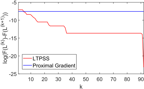
Figure 2 shows an example plot of log(F(L(k) ) - F(L(k+1) )) for the proposed KM algorithm in one run that converges at the 92-nd iteration. Since log(F(L(k) ) - F(L(k+1) )) decreases in a step-wise way until convergence, the KM algorithm enjoys considerable constant-step descents. Other runs of the KM algorithm also have similar plots. In order to make comparison, we remove the constraint ∥L∥2 ⩽ 1 so that the general proximal gradient method could be applied, which may be the closest method to the KM algorithm. The plot of the proximal gradient algorithm is also shown in Figure 2, which indicates a worse convergence rate than the KM algorithm.
4 Experimental Results
We follow the experimental framework of [Kelly et al., 2023a; Lai and Yang, 2023; Lai et al., 2024] to evaluate the performance of the proposed LTPSS. The experimental settings and more experimental results are put in Supplementary A.5.
4.1 Mean Return
At the t-th trading time, a trading strategy determines an LTP ˆLt+1 for the next trading time. Then the return of this strategy for the next trading time can be computed by rt+1 := S⊤ t ˆLt+1Rt+1. Suppose there are T trading times in total. Then the mean return (MR) of this strategy is MR := 1 T ∑Tt=1 rt. It reflects the average investing gain of a trading strategy during the whole investment. The MRs of different trading strategies on the 7 benchmark data sets are shown in Table 1. It indicates that LTP-PP performs well on the FF25 data sets, which are well interpreted by the Fama-French five factors. But it deteriorates on the other data sets collected in diverse financial circumstances. For example, LTP-PP suffers a negative MR on Stoxx50, which represents a financial market outside US. LTP-SF also performs badly with negative MRs on MSCI, Stoxx50, FOF, and FTSE100, which indicates that using only the own signal of each asset is ineffective. SDCP has similar bad performance as LTP-SF, since it cannot achieve full-reinvestment on each trade. mSSRMPGA has relatively lowMRs because it is a uni-linear trading strategy without an effective signal learning scheme. LTPSS achieves the best MRs on most data sets except MSCI where it is slightly worse than LTP-CF, hence more PPs may not necessarily lead to better performance. It achieves greater advantage over LTP-SF and LTP-PP on MSCI, Stoxx50, FOF, and FTSE100. For example, it performs about 1, 2, and 25 times better than LTP-PP on MSCI, FOF, and FTSE100, respectively. These results indicate that LTPSS can extract key features from the prediction matrix and performs robustly in diverse financial circumstances.
4.2 Sharpe Ratio
The Sharpe ratio (SR, [Sharpe, 1966]) is a widely-used evaluating metric for the risk-adjusted return of a trading strategy.
It can be calculated as follows in the framework of this paper: SR := MR-rf ˆ s(rt) , where rf is the average risk-free return during the investment, and ˆ s(·) is the sample standard deviation operator. The SR need not be annualized and this does not affect the assessment. rf is given on the FF25 data sets but not given on MSCI, Stoxx50, FOF, and FTSE100. Hence we set rf = 0 for the latter 4 data sets. The SRs of different trading strategies are shown in Table 1. Again, SDCP, LTPSF, and mSSRM-PGA have similar bad performance due to ineffective investing schemes. LTP-PP outperforms LTP-CF on FF25BM and FF25MEINV, but it still performs badly on Stoxx50 and FTSE100. It indicates that the first few PPs may not be robust enough to different financial circumstances.
LTPSS achieves the best SRs on all the data sets, especially on Stoxx50, FOF and FTSE100 where it keeps up robust performance. The advantage of LTPSS over LTP-CF and LTPPP is large on Stoxx50. These results indicate that LTPSS is effective and robust in balancing investing return and risk.
4.3 Information Ratio
In finance, it is conventional to factorize the return of a trading strategy for in-depth analysis of its composition. Following [Kelly et al., 2023a], we adopt the following Fama-French five-factor model:
where rt and rSF,t denote the returns on the t-th trading time of a trading strategy and the LTP-SF strategy, respectively. MKT (market), SMB (size), HML (value), RMW (profitability), and CMA (investment) denote the Fama-French five factors. ζ0 ∼ ζ5 are the coefficients of the corresponding factors. εt is the residue for this regression model. α [Lintner, 1965] can be seen as the pure return of the trading strategy excluding all the above-mentioned factors, which will be further investigated in Section 4.4. After conducting a regression for (34), estimations for ˆα and ˆ s(εt) can be obtained. The information ratio (IR, [Treynor and Black, 1973]) is another widely-used risk-adjusted return: IR := ˆα ˆ s(εt) . It can be seen as the pure SR hedging out all the above-mentioned factors. Note that the return of LTP-SF has also been hedged out in (34), thus LTPSF does not have IRs itself. As for other trading strategies, a positive IR can be roughly considered as a better performance than LTP-SF. Table 1 shows the IRs of different trading strategies. LTP-PP performs well on the FF25 data sets but deteriorates on MSCI, Stoxx50, and FTSE100. In comparison, LTPSS outperforms LTP-CF and LTP-PP on all the data sets, especially on MSCI and Stoxx50 where it achieves effective and robust performance. These results also show its good ability in balancing return and risk.
4.4 α Factor
α represents the pure return of a trading strategy based on the market-neutral perspective, since it hedges out all the marketrelated factors. It measures the intrinsic return that is brought by the traded assets themselves instead of the market volatility. It is widely employed to evaluate the effectiveness of a trading strategy despite the market effect. Along with the regression for (34), a left-tailed t-test can be conducted to obtain the p-value for the corresponding α. Both αs and p-values of different trading strategies are presented in Table 1. SDCP and mSSRM-PGA perform badly on all the data sets. Similar to the results of IR, LTP-PP performs badly on MSCI, Stoxx50, and FTSE100. In comparison, LTPSS achieves the best performance on all the data sets. Hence LTPSS is effective in achieving pure returns.
| Eval. | Strategy | FF25BM | FF25MEINV | FF25MEOP | MSCI | Stoxx50 | FOF | FTSE100 |
|---|---|---|---|---|---|---|---|---|
| SDCP | 0.0121 | 0.0110 | 0.0111 | -0.0126 | -0.0087 | -0.0015 | -0.0795 | |
| MR | LTP-SF | 0.0120 | 0.0107 | 0.0109 | -0.0170 | -0.0097 | -0.0017 | -0.0274 |
| LTP-CF | 0.0133 | 0.0137 | 0.0130 | 0.0090 | 0.0004 | 0.0022 | 0.0242 | |
| LTP-PP | 0.0129 | 0.0133 | 0.0126 | 0.0041 | -0.0004 | 0.0012 | 0.0013 | |
| mSSRM-PGA | 0.0006 | 0.0006 | 0.0006 | -0.0003 | -0.0003 | 0.0006 | 0.0036 | |
| LTPSS | 0.0133 | 0.0143 | 0.0134 | 0.0087 | 0.0012 | 0.0030 | 0.0273 | |
| SR | SDCP | 0.1429 | 0.1522 | 0.1626 | -0.2702 | -0.0738 | -0.0254 | -0.2802 |
| LTP-SF | 0.1356 | 0.1394 | 0.1509 | -0.2918 | -0.0738 | -0.0280 | -0.0941 | |
| LTP-CF | 0.2010 | 0.2590 | 0.2535 | 0.2257 | 0.0070 | 0.0659 | 0.1359 | |
| LTP-PP | 0.2049 | 0.2642 | 0.1998 | 0.1743 | -0.0091 | 0.0312 | 0.0114 | |
| mSSRM-PGA | 0.0691 | 0.0683 | 0.0693 | -0.0277 | -0.0214 | 0.0413 | 0.1253 | |
| LTPSS | 0.2049 | 0.2731 | 0.2619 | 0.2445 | 0.0198 | 0.0874 | 0.1521 | |
| IR | SDCP | 0.1407 | 0.2103 | 0.1645 | 0.0088 | 0.0922 | 0.0613 | -0.1957 |
| LTP-CF | 0.1567 | 0.2203 | 0.1938 | 0.1064 | -0.0084 | 0.1060 | 0.1314 | |
| LTP-PP | 0.1489 | 0.2308 | 0.1715 | -0.0203 | -0.0365 | 0.1060 | -0.0468 | |
| mSSRM-PGA | 0.0852 | 0.0839 | 0.0854 | -0.0368 | -0.0329 | 0.0417 | 0.1320 | |
| LTPSS | 0.1650 | 0.2418 | 0.2047 | 0.1366 | 0.0053 | 0.1409 | 0.1503 | |
| α | SDCP | 0.0006 | 0.0009 | 0.0007 | 0.0001 | 0 | 0.0002 | 0 |
| LTP-CF | 0.0063 | 0.0081 | 0.0067 | 0.0038 | -0.0005 | 0.0028 | 0.0229 | |
| LTP-PP | 0.0054 | 0.0079 | 0.0056 | -0.0004 | -0.0015 | 0.0022 | -0.0050 | |
| mSSRM-PGA | 0.0006 | 0.0005 | 0.0005 | -0.0004 | -0.0004 | 0.0005 | 0.0033 | |
| LTPSS | 0.0063 | 0.0087 | 0.0067 | 0.0043 | 0.0003 | 0.0036 | 0.0264 | |
| p-val. | SDCP | 0.0007 | 0 | 0.0001 | 0.4700 | 0.0284 | 0.2536 | 0.0263 |
| LTP-CF | 0.0002 | 0 | 0 | 0.1807 | 0.5846 | 0.1260 | 0.1794 | |
| LTP-PP | 0.0002 | 0 | 0 | 0.5694 | 0.8228 | 0.1260 | 0.8140 | |
| mSSRM-PGA | 0 | 0 | 0 | 0.1176 | 0.0201 | 0.0733 | 0.0002 | |
| LTPSS | 0.0001 | 0 | 0 | 0.1210 | 0.4468 | 0.0643 | 0.1471 | |
| MDD | SDCP | 0.8700 | 0.7805 | 0.6695 | 0.7010 | 1.0000 | 0.4311 | 0.9685 |
| LTP-SF | 0.8858 | 0.8083 | 0.6857 | 0.7917 | 1.0000 | 0.4572 | 0.9895 | |
| LTP-CF | 0.7131 | 0.5309 | 0.5188 | 0.3955 | 0.8944 | 0.1983 | 0.5986 | |
| LTP-PP | 0.6530 | 0.5078 | 0.5208 | 0.1453 | 0.7780 | 0.2188 | 0.4017 | |
| mSSRM-PGA | 0.6237 | 0.4834 | 0.4958 | 0.5294 | 0.8676 | 0.5454 | 0.4596 | |
| LTPSS | 0.6918 | 0.5184 | 0.5259 | 0.3295 | 0.8126 | 0.1894 | 0.5141 |
4.5 MaximumDrawdown
The maximum drawdown (MDD, [Magdon-Ismail and Atiya, 2004]) measures the maximum percentage loss of wealth from a past peak to a past valley for a PO method, which corresponds to the worst case in the investment. It is mainly treated by a back-end risk control mechanism, such as setting stop loss orders. For a reference purpose, we present MDDs of different trading strategies in Table 1. LTPSS achieves competitive MDDs, roughly between those of LTP-PP and LTP-CF. Since LTPSS achieves the best performance in most cases with other evaluating metrics, it is an effective method considering both return and risk.
5 Conclusion
In this work, we propose a linear trading position with sparse spectrum (LTPSS) that can explore a larger spectral region of the prediction matrix and extract key features from it. Our approach improves on the existing principal portfolio (PP) strategy that it allows for all the PPs with flexible spectral energies. We develop a Krasnosel'ski˘ı-Mann fixed-point algorithm to solve the proposed optimization model, which is able to handle the complicated geometric structure of the constraint and the nuclear norm regularization. It also guarantees a linear convergence and the descent property of the objective values. Experimental results show that LTPSS achieves competitive and robust investing performance in diverse financial circumstances according to some common evaluating metrics.
A direct impact of LTPSS is to provide a novel trading strategy for the interdiscipline of machine learning and financial technology. It is highly interpretable and understandable in the general framework of finance, as well as tractable and reliable with theoretical guarantees. It can enrich the factor library for quantitative research, or reveal some intrinsic patterns of the asset pool. A possible limitation is that LTPSS may not be applied to nonlinear trading frameworks, which is partly due to the lack of such trading frameworks in finance. As for future works, we can extend LTPSS to more general factor trading architectures, or develop a nonlinear trading position that has a stronger signal processing ability. Exploring the relationship between PPs and conventional financial factors is also an interesting topic.
Acknowledgments
This work is supported in part by the National Natural Science Foundation of China under grants 62176103 and 72173141, in part by the Guangdong Basic and Applied Basic Research Foundation under grant 2024A1515010749, and in part by the Science and Technology Planning Project of Guangzhou under grant 2024A04J9896.
@inproceedings{ijcai2025p618,
  title     = {Linear Trading Position with Sparse Spectrum},
  author    = {Lai, Zhao-Rong and Yang, Haisheng},
  booktitle = {Proceedings of the Thirty-Fourth International Joint Conference on
               Artificial Intelligence, {IJCAI-25}},
  publisher = {International Joint Conferences on Artificial Intelligence Organization},
  editor    = {James Kwok},
  pages     = {5554--5562},
  year      = {2025},
  month     = {8},
  note      = {Main Track},
  doi       = {10.24963/ijcai.2025/618},
  url       = {https://doi.org/10.24963/ijcai.2025/618},
}
TY - CPAPER TI - Linear Trading Position with Sparse Spectrum AU - Lai, Zhao-Rong AU - Yang, Haisheng T2 - Proceedings of the Thirty-Fourth International Joint Conference on Artificial Intelligence, IJCAI-25 PB - International Joint Conferences on Artificial Intelligence Organization PY - 2025 SP - 5554 EP - 5562 DO - 10.24963/ijcai.2025/618 UR - https://doi.org/10.24963/ijcai.2025/618 ER -Copied
Machine-readable versions of this paper, for tools and AI agents:





