
Conditional Information Bottleneck-Based Multivariate Time Series Forecasting
Proceedings of the Thirty-Fourth International Joint Conference on Artificial Intelligence. Main Track. Pages 5634-5642.
https://doi.org/10.24963/ijcai.2025/627
Keywords
- Machine Learning: ML: Time series and data streams
- Data Mining: DM: Mining spatial and/or temporal data
- Machine Learning: ML: Sequence and graph learning
- Data Mining: DM: Mining data streams
Abstract
Multivariate time series (MTS) forecasting endeavors to anticipate the forthcoming sequence of interdependent variables through the utilization of past observations. The prevailing methodologies, relying on deep neural networks, Transformer, or information bottleneck frameworks, persist in confronting challenges such as overlooking or inadequately capturing the inter / intra-series correlations evident in practical MTS datasets. In response to these challenges, we introduce a conditional information bottleneck-based strategy for MTS forecasting, grounded in information theory. Initially, we establish a conditional information bottleneck principle to capture the inter-series correlations via conditioning on non-target variables. Subsequently, a conditional mutual information-based technique is introduced to extract intra-series correlations by conditioning historical data, ensuring temporal consistency within each variable. Lastly, we devise a unified optimization objective and propose a training algorithm to collectively capture inter / intra-series correlations. Empirical investigations on authentic datasets underscore the superiority of our proposed approach over other cutting-edge competitors. Our code is available at https:
//github.com/Xinhui-Lee/CIB-MTSF.
- MAE 24 1.250 0.638 3.135 1.201 1.305 0.767 2.215 1.081 3.040 1.186 2.441 1.058 4.247 1.355 4.657 1.449 4.268 1.385 36 1.299 0.650 3.355 1.215 1.428 0.763 1.963 0.963 3.356 1.230 2.469 1.028 4.064 1.332 4.650 1.463 4.768 1.494 48 1.220 0.644 3.588 1.306 1.233 0.798 1.673 0.854 3.441 1.223 2.430 1.037 4.559 1.440 5.004 1.542 5.333 1.592 ILI 60 1.351 0.710 3.590 1.331 1.496 0.853 2.368 1.096 3.608 1.302 2.457 1.065 5.346 1.648 5.071 1.543 5.083 1.556 96 0.148 0.195 0.161 0.220 0.153 0.209 0.176 0.237 0.153 0.217 0.161 0.226 0.169 0.219 0.354 0.405 0.161 0.223 192 0.194 0.237 0.204 0.257 0.200 0.249 0.220 0.282 0.197 0.269 0.220 0.283 0.197 0.238 0.419 0.434 0.206 0.278 336 0.243 0.275 0.254 0.291 0.251 0.287 0.265 0.319 0.252 0.311 0.275 0.328 0.257 0.285 0.583 0.543 0.261 0.322 Weather 720 0.311 0.327 0.334 0.344 0.321 0.337 0.323 0.362 0.318 0.363 0.323 0.356 0.315 0.327 0.916 0.705 0.324 0.366 96 0.390 0.273 0.576 0.357 0.405 0.286 0.410 0.282 0.512 0.290 0.508 0.301 0.520 0.338 0.733 0.410 0.527 0.316 192 0.394 0.281 0.602 0.366 0.416 0.288 0.423 0.287 0.523 0.297 0.536 0.315 0.579 0.367 0.777 0.435 0.534 0.320 336 0.418 0.287 0.621 0.370 0.428 0.297 0.436 0.296 0.530 0.300 0.525 0.310 0.616 0.419 0.776 0.434 0.540 0.335 Traffic 720 0.447 0.305 0.633 0.374 0.461 0.314 0.466 0.315 0.573 0.313 0.571 0.323 0.689 0.452 0.827 0.466 0.557 0.343 96 0.130 0.221 0.143 0.252 0.137 0.241 0.140 0.237 0.187 0.283 0.159 0.267 0.161 0.257 0.304 0.393 0.198 0.294 192 0.147 0.235 0.166 0.271 0.152 0.246 0.153 0.249 0.258 0.330 0.168 0.279 0.170 0.265 0.327 0.417 0.266 0.339 336 0.167 0.258 0.176 0.281 0.171 0.267 0.169 0.267 0.323 0.369 0.196 0.308 0.188 0.280 0.333 0.422 0.328 0.373 Electricity 720 0.201 0.285 0.252 0.367 0.212 0.296 0.203 0.301 0.404 0.423 0.203 0.312 0.223 0.309 0.351 0.427 0.422 0.410 96 0.361 0.388 0.422 0.439 0.373 0.398 0.375 0.399 0.386 0.429 0.396 0.427 0.398 0.414 0.941 0.769 0.439 0.461 192 0.383 0.407 0.449 0.459 0.412 0.420 0.405 0.416 0.419 0.444 0.430 0.453 0.468 0.453 1.007 0.786 0.476 0.477 336 0.385 0.409 0.461 0.466 0.392 0.417 0.439 0.443 0.440 0.461 0.433 0.458 0.566 0.512 1.038 0.784 0.736 0.643 ETTh1 720 0.420 0.443 0.499 0.501 0.448 0.463 0.472 0.490 0.519 0.524 0.474 0.508 0.740 0.650 1.144 0.857 0.916 0.750 96 0.260 0.326 0.355 0.401 0.267 0.332 0.289 0.353 0.628 0.563 0.289 0.357 0.377 0.426 1.549 0.952 0.690 0.614 192 0.314 0.365 0.407 0.432 0.317 0.367 0.383 0.418 0.703 0.624 0.409 0.438 0.619 0.639 3.792 1.542 0.745 0.662 336 0.302 0.365 0.391 0.423 0.306 0.367 0.448 0.465 0.827 0.675 0.417 0.452 0.849 0.805 4.215 1.642 0.886 0.721 ETTh2 720 0.374 0.418 0.406 0.442 0.390 0.421 0.605 0.551 1.181 0.840 0.426 0.473 0.874 0.679 3.656 1.619 1.299 0.936 96 0.289 0.337 0.303 0.360 0.291 0.341 0.299 0.343 0.316 0.373 0.314 0.360 0.323 0.360 0.626 0.560 0.428 0.446 192 0.327 0.360 0.353 0.391 0.332 0.364 0.335 0.365 0.377 0.411 0.359 0.387 0.346 0.376 0.725 0.619 0.509 0.491 336 0.361 0.383 0.379 0.408 0.363 0.385 0.369 0.386 0.431 0.442 0.398 0.413 0.395 0.404 1.005 0.741 0.577 0.556 ETTm1 720 0.413 0.417 0.429 0.437 0.424 0.417 0.425 0.421 0.600 0.547 0.459 0.464 0.493 0.470 1.133 0.845 0.713 0.729 96 0.160 0.247 0.186 0.273 0.162 0.254 0.167 0.260 0.421 0.461 0.178 0.273 0.174 0.265 0.355 0.462 0.463 0.503 192 0.213 0.285 0.249 0.314 0.213 0.289 0.224 0.303 0.503 0.519 0.245 0.316 0.234 0.310 0.595 0.586 0.530 0.547 336 0.266 0.321 0.301 0.347 0.275 0.331 0.281 0.342 0.611 0.580 0.295 0.350 0.352 0.397 1.270 0.871 0.449 0.473 ETTm2 720 0.349 0.373 0.401 0.407 0.355 0.380 0.397 0.421 0.996 0.750 0.389 0.406 0.911 0.671 3.001 1.267 1.093 0.836 96 0.079 0.195 0.102 0.230 0.089 0.210 0.088 0.218 0.188 0.365 0.102 0.235 0.108 0.236 0.847 0.752 0.208 0.381 192 0.164 0.288 0.195 0.317 0.173 0.297 0.176 0.315 0.456 0.532 0.172 0.316 0.212 0.343 1.204 0.895 0.459 0.512 336 0.304 0.396 0.360 0.436 0.322 0.408 0.313 0.427 0.796 0.741 0.272 0.407 0.394 0.468 1.672 1.036 0.710 0.698 Exchange 720 0.769 0.655 0.940 0.738 0.867 0.701 0.839 0.695 1.367 0.943 0.714 0.658 1.398 1.102 2.478 1.310 1.323 0.912
- [Adebiyi et al., 2014] Ayodele A. Adebiyi, Aderemi O. Adewumi, and Charles K. Ayo. Stock Price Prediction Using the ARIMA Model. In Proceedings of the 16th In- ternational Conference on Computer Modelling and Sim- ulation (ICCM), pages 106-112, 2014.
- [Belghazi et al., 2018] Mohamed Ishmael Belghazi, Aristide Baratin, Sai Rajeshwar, Sherjil Ozair, Yoshua Bengio, Aaron Courville, and R Devon Hjelm. Mutual Informa- tion Neural Estimation. In Proceedings of the 35th Inter- national Conference on Machine Learning (ICML), vol- ume 80, pages 531-540, 2018.
- [Cai et al., 2024] Wanlin Cai, Yuxuan Liang, Xianggen Liu, Jianshuai Feng, and Yuankai Wu. MSGNet: Learn- ing Multi-Scale Inter-Series Correlations for Multivariate Time Series Forecasting. In Proceedings of the 38th AAAI Conference on Artificial Intelligence (AAAI), volume 38, pages 11141-11149, 2024.
- [Chen et al., 2023] Shengchao Chen, Guodong Long, Tao Shen, and Jing Jiang. Prompt Federated Learning for Weather Forecasting: Toward Foundation Models on Me- teorological Data. In Proceedings of the 32nd Interna- tional Joint Conference on Artificial Intelligence (IJCAI), pages 3532-3540, 2023. IJCAI
- [Choi and Lee, 2024] MinGyu Choi and Changhee Lee. Conditional Information Bottleneck Approach for Time Series Imputation. In Proceedings of the 12th Interna- tional Conference on Learning Representations (ICLR), 2024.
- [Duan et al., 2024] Liang Duan, Xiang Chen, Wenjie Liu, Daliang Liu, Kun Yue, and Angsheng Li. Structural En- tropy Based Graph Structure Learning for Node Classifi- cation. In Proceedings of the 38th AAAI Conference on Ar- tificial Intelligence (AAAI), volume 38, pages 8372-8379, 2024.
- [Grzegorz, 2023] Dudek Grzegorz. STD: A Seasonal-Trend- Dispersion Decomposition of Time Series. IEEE Transac- tions on Knowledge and Data Engineering, 35(10):10339- 10350, 2023.
- [He et al., 2024] Shiming He, Genxin Li, Kun Xie, and Pradip Kumar Sharma. Fusion Graph Structure Learning- Based Multivariate Time Series Anomaly Detection with Structured Prior Knowledge. IEEE Transactions on Infor- mation Forensics and Security, 19:8760-8772, 2024.
- [Huang et al., 2024] Qihe Huang, Lei Shen, Ruixin Zhang, Jiahuan Cheng, Shouhong Ding, Zhengyang Zhou, and Yang Wang. HDMixer: Hierarchical Dependency with Extendable Patch for Multivariate Time Series Forecast- ing. In Proceedings of the 38th AAAI Conference on Artifi- cial Intelligence (AAAI), volume 38, pages 12608-12616, 2024.
- [Kullback, 1997] Solomon Kullback. Information theory and statistics. Courier Corporation, 1997.
- [Li et al., 2022] Longyuan Li, Junchi Yan, Yunhao Zhang, Jihai Zhang, Jie Bao, Yaohui Jin, and Xiaokang Yang. Learning Generative RNN-ODE for Collaborative Time- Series and Event Sequence Forecasting. IEEE Transac- tions on Knowledge and Data Engineering, 35(7):7118- 7137, 2022.
- [Li et al., 2023] Yifan Li, Xiaoyan Peng, Jia Zhang, Zhiy- ong Li, and Ming Wen. DCT-GAN: Dilated Convolutional Transformer-Based GAN for Time Series Anomaly Detec- tion. IEEE Transactions on Knowledge and Data Engi- neering, 35(4):3632-3644, 2023.
- [Li et al., 2024] Ruohan Li, Yiqun Xie, Xiaowei Jia, Dong- dong Wang, Yanhua Li, Yingxue Zhang, Zhihao Wang, and Zhili Li. SolarCube: An Integrative Benchmark Dataset Harnessing Satellite and In-situ Observations for Large-scale Solar Energy Forecasting. In Proceedings of the 37th Advances in Neural Information Processing Sys- tems (NIPS), 2024.
- [Liu et al., 2024] Yong Liu, Tengge Hu, Haoran Zhang, Haixu Wu, Shiyu Wang, Lintao Ma, and Mingsheng Long. iTransformer: Inverted Transformers Are Effective for Time Series Forecasting. In Proceedings of the 12th Inter- national Conference on Learning Representations (ICLR), 2024.
- [Liu, 2022] Guangcan Liu. Time Series Forecasting Via Learning Convolutionally Low-Rank Models. IEEE Transactions on Information Theory, 68(5):3362-3380, 2022.
- [Ma et al., 2024] Xiang Ma, Xuemei Li, Lexin Fang, Tian- long Zhao, and Caiming Zhang. U-Mixer: An Unet-Mixer Architecture with Stationarity Correction for Time Series Forecasting. In Proceedings of the 38th AAAI Confer- ence on Artificial Intelligence (AAAI), volume 38, pages 14255-14262, 2024.
- [Nie et al., 2023] Yuqi Nie, Nam H. Nguyen, Phanwadee Sinthong, and Jayant Kalagnanam. A Time Series is Worth 64 Words: Long-Term Forecasting with Transform- ers. In Proceedings of the 11th International Conference on Learning Representations (ICLR), 2023.
- [Oord et al., 2018] Aaronvanden Oord, Yazhe Li, and Oriol Vinyals. Representation Learning with Contrastive Predic- tive Coding. In arXiv preprint, volume arXiv:1807.03748, 2018.
- [Pagliarini et al., 2024] Giovanni Pagliarini, Simone Scaboro, Giuseppe Serra, Guido Sciavicco, and Ionel Ed- uard Stan. Neural-Symbolic Temporal Decision Trees for Multivariate Time Series Classification. Information and Computation, 301:105209, 2024.
- [Ryabko, 2019] Daniil Ryabko. Time-Series Information and Unsupervised Learning of Representations. IEEE Transactions on Information Theory, 66(3):1702-1713, 2019.
- [Sun et al., 2023] Le Sun, Chenyang Li, Bo Liu, and Yanchun Zhang. Class-Driven Graph Attention Net- work for Multi-Label Time Series Classification in Mobile Health Digital Twins. IEEE Journal on Selected Areas in Communications, 41(10):3267-3278, 2023.
- [Tian et al., 2020] Yonglong Tian, Dilip Krishnan, and Phillip Isola. Contrastive Multiview Coding. In Proceed- ings of the 16th European Conference on Computer Vision (ECCV), pages 776-794, 2020.
- [Tishby et al., 2000] Naftali Tishby, Fernando C. Pereira, and William Bialek. The information bottleneck method. In arXiv preprint, volume physics/0004057, 2000.
- [Wang et al., 2022a] Zhiyuan Wang, Xovee Xu, Goce Tra- jcevski, Kunpeng Zhang, Ting Zhong, and Fan Zhou. PrEF: Probabilistic electricity forecasting via Copula- augmented state space model. In Proceedings of the 36th AAAI Conference on Artificial Intelligence (AAAI), vol- ume 36, pages 12200-12207, 2022.
- [Wang et al., 2022b] Zhiyuan Wang, Xovee Xu, Weifeng Zhang, Goce Trajcevski, Ting Zhong, and Fan Zhou. Learning Latent Seasonal-Trend Representations for Time Series Forecasting. In Proceedings of the 35th Advances in Neural Information Processing Systems (NIPS), pages 38775-38787, 2022.
- [Wang et al., 2023] Huiqiang Wang, Jian Peng, Feihu Huang, Jince Wang, Junhui Chen, and Yifei Xiao. MICN: Multi-Scale Local and Global Context Modeling for Long- Term Series Forecasting. In Proceedings of the 11th Inter- national Conference on Learning Representations (ICLR), 2023.
- [Wu et al., 2020] Zonghan Wu, Shirui Pan, Guodong Long, Jing Jiang, Xiaojun Chang, and Chengqi Zhang. Connect- ing the Dots: Multivariate Time Series Forecasting With Graph Neural Networks. In Proceedings of the 26th ACM SIGKDD International Conference on Knowledge Discov- ery and Data Mining (SIGKDD), pages 753-763, 2020.
- [Wu et al., 2021] Haixu Wu, Jiehui Xu, Jianmin Wang, and Mingsheng Long. Autoformer: Decomposition Trans- formers with Auto-Correlation for Long-Term Series Fore- casting. In Proceedings of the 34th Advances in Neu- ral Information Processing Systems (NIPS), pages 22419- 22430, 2021.
- [Yang et al., 2024] Yingnan Yang, Qingling Zhu, and Jiany- ong Chen. VCformer: Variable Correlation Transformer with Inherent Lagged Correlation for Multivariate Time Series Forecasting. In Proceedings of the 33rd Interna- tional Joint Conference on Artificial Intelligence (IJCAI), 2024. IJCAI
- [Yi et al., 2023] Kun Yi, Qi Zhang, Wei Fan, Shoujin Wang, Pengyang Wang, Hui He, Ning An, Defu Lian, Longbing Cao, , and Zhendong Niu. Frequency-Domain MLPs are More Effective Learners in Time Series Forecasting. In Proceedings of the 36th Advances in Neural Information Processing Systems (NIPS), 2023.
- [Yi et al., 2024] Kun Yi, Qi Zhang, Hui He, Kaize Shi, Liang Hu, Ning An, and Zhendong Niu. Deep Coupling Network For Multivariate Time Series Forecasting. ACM Transac- tions on Information Systems, 42(5):1-28, 2024.
- [Zeng et al., 2023] Ailing Zeng, Muxi Chen, Lei Zhang, and Qiang Xu. Are Transformers Effective for Time Series Forecasting?. In Proceedings of the 37th AAAI Confer- ence on Artificial Intelligence (AAAI), volume 37, pages 11121-11128, 2023.
- [Zhang and Yan, 2023] Yunhao Zhang and Junchi Yan. Crossformer: Transformer Utilizing Cross-Dimension De- pendency for Multivariate Time Series Forecasting. In Proceedings of the 11th International Conference on Learning Representations (ICLR), 2023.
- [Zhou et al., 2023] Haoyi Zhou, Jianxin Li, Shanghang Zhang, Shuai Zhang, Mengyi Yan, and Hui Xiong. Ex- panding the Prediction Capacity in Long Sequence Time- Series Forecasting. Artificial Intelligence, 318:103886, 2023.
- [Zhou et al., 2024] Ziyu Zhou, Gengyu Lyu, Yiming Huang, Zihao Wang, Ziyu Jia, and Zhen Yang. SDformer: Trans- former with Spectral Filter and Dynamic Attention for Multivariate Time Series Long-term Forecasting. In Pro- ceedings of the 33rd International Joint Conference on Ar- tificial Intelligence (IJCAI), 2024. IJCAI
References were extracted automatically from the PDF and may contain errors.
Full text extracted automatically from the PDF; figures, tables and equations may differ. The PDF is the version of record.
1 Introduction
Multivariate time series (MTS) forecasting, a focal point in domains such as stock price [Adebiyi et al., 2014], energy management [Li et al., 2024], and weather prediction [Chen et al., 2023], necessitates capturing inter-series correlations that delineate dependencies among variables at the same time and intra-series correlations that signify temporal dependencies within a variable across different time spans. For instance, in weather forecasting, grasping inter-series correlations is critical for deciphering the intertwined relationships among temperature, humidity, and vapor pressure. Higher temperatures induce increased evaporation, resulting in elevated humidity levels and altered vapor pressure. Furthermore, capturing intra-series correlations preserves the temporal coherence of each variable across adjacent time periods, facilitating gradual transitions in temperature between day and night or across seasons.
∗Corresponding author.
Existing methods utilize deep neural networks, including recurrent neural networks (RNN) [Pagliarini et al., 2024], convolutional neural networks (CNN) [Sun et al., 2023], graph convolutional networks (GCN) [He et al., 2024], and multilayer perceptrons (MLP) [Zeng et al., 2023] for MTS forecasting. These approaches often encounter challenges in maintaining temporal coherence due to struggles in capturing long-term dependencies and insensitivity to temporal order. Transformer-based methods [Zhou et al., 2023; Nie et al., 2023] leverage self-attention mechanisms for MTS forecasting. However, they lack interpretability in capturing inter-variable dependencies.
The Information Bottleneck (IB) principle, aimed at retaining relevant information for forecasting while reducing irrelevant information [Tishby et al., 2000], has been applied in IB-based models like LaST and DeepCoupling [Wang et al., 2022b; Yi et al., 2024] to identify temporal patterns while preserving essential forecasting information. However, the exploration of leveraging IB to capture variable dependencies and maintain temporal coherence remains uncharted. Establishing a model that incorporates the IB principle to effectively capture inter / intra-series correlations remains a valuable pursuit.
The conditional information bottleneck (CIB) method integrates task-relevant background information using mutual information through conditional variables, aiming to minimize redundancy while capturing useful information from all data [Choi and Lee, 2024]. Hence, we employ CIB to discern intricate interaction patterns among variables within each time period. Subsequently, to ensure temporal coherence within each variable across neighboring periods, we utilize conditional mutual information (CMI) to preserve the inherent sequence consistency. Addressing the efficient calculation of mutual information and precise representation of correlations in MTS involves tackling the following two pivotal challenges:
- How can the CIB-based principle be formulated to capture inter-series correlations in MTS data?
- How can CMI be utilized to capture intra-series correla-
tions and ensure continuous time coherence?
For the first challenge, we employ CIB to diminish superfluous data while conserving pertinent information for MTS forecasting. To delineate inter-series dependencies, each variable is considered with other variables as conditions, offering additional temporal insights. To streamline mutual information computation within CIB, we establish manageable upper and lower bounds for each mutual information component. Subsequently, we formulate the CIB-based loss function by amalgamating the estimated mutual information terms.
For the second issue, we segment the time series into overlapping patches to enhance the capture of local intra-series correlations within each variable. To preserve the temporal coherence without disrupting the continuity of the time series segmentation, we introduce the CMI-based principle, where all preceding patches are regarded as conditions to offer additional temporal insights. To address the computational intensity of mutual information estimation within CMI, we establish a lower bound for mutual information approximation, subsequently defining the CMI-based loss function.
Ultimately, we introduce a cohesive objective by amalgamating the CIB and CMI-based loss functions to collectively capture inter / intra-series correlations within MTS data. Additionally, we present a training algorithm tailored to MTS data, offering a systematic approach to capturing intervariable dependencies and upholding temporal coherence.
We summarize our contributions as follows:
- We propose the CIB-based principle for MTS forecasting to delineate inter-variable dependencies within concurrent time periods.
- We introduce the CMI-based approach for MTS forecasting to ensure temporal consistency within individual variables across neighboring time segments.
- We present a unified optimization goal and training protocol to concurrently capture both inter / intra-series correlations.
- We conduct extensive experiments on authentic datasets and demonstrate the superior efficacy of our method over state-of-the-art alternatives.
2 RelatedWork
Deep neural network-enabled MTS forecasting. Diverse deep neural network methodologies have emerged for MTS forecasting. RNN-based architectures leverage hidden states to capture temporal dependencies [Li et al., 2022; Pagliarini et al., 2024]. CNN-based models extract local features and recurrent patterns through convolutions [Sun et al., 2023; Wang et al., 2023]. Graph structure is instrumental in capturing intricate dependencies in data [Duan et al., 2024], and thus GCN-based models establish graph structures from MTS, employing graph convolutions to propagate temporal features across nodes [He et al., 2024; Wu et al., 2020]. MLP models are tailored for efficient MTS forecasting [Zeng et al., 2023]. Certain models extract local temporal features by segmenting time series into patches [Huang et al., 2024; Ma et al., 2024]. Nevertheless, these approaches may struggle to capture dependencies over extended periods and might overlook the sequential nature of temporal data, potentially compromising the preservation of long-term patterns crucial for accurate forecasting.
Transformer-based MTS forecasting. To mitigate computational overhead, Zhou et al. [Zhou et al., 2023] introduce Informer, employing ProbSparse attention, while Li et al. [Li et al., 2023] integrate dilated convolutional networks and Transformer blocks to circumvent global attention computations. Liu et al. [Liu et al., 2024] captures inter-variable dependencies by applying self-attention over variate tokens. Strategies such as frequency domain transformation or time series decomposition aid in extracting periodic and global features, easing computational demands [Wu et al., 2021; Zhou et al., 2024]. Techniques like fragmentation [Nie et al., 2023] or multi-scale processing [Zhang and Yan, 2023] of time series, which capture both local and global dependencies. Nonetheless, these approaches lack the interpretability of inter-variable dependencies.
Temporal pattern recognition-based MTS forecasting. Several methods leverage frequency-domain transformations to uncover global and periodic trends in MTS, facilitating the detection of short-term variations and long-term relationships [Yi et al., 2023; Cai et al., 2024]. For instance, Wang et al. [Wang et al., 2022b] utilize mutual information for disentangled representation learning, while Grzegorz et al. [Grzegorz, 2023] decompose MTS into trend and seasonality components to discern distinct patterns. Yi et al. [Yi et al., 2024] identify multi-order dependency patterns and the coupling of MTS through Information Bottleneck (IB) principles. Choi et al. [Choi and Lee, 2024] addresses the issue of overly stringent regularization in IB by introducing conditional regularization based on temporal contexts within time series. Additionally, Liu [Liu, 2022] reduces data dimensions while preserving pertinent patterns in lengthy time series. Ryabko [Ryabko, 2019] maps high-dimensional time series into finite spaces to uncover underlying dependencies accurately. Nevertheless, these approaches struggle with the interpretation of complex multivariate interactions.
3 Preliminaries and ProblemFormalization
In this section, we present formulations of MTS forecasting and conditional information bottleneck.
MTS forecasting. Given L historical time steps of N variables, the input series is denoted as X = {X1,X2, . . . ,XN} ∈ RN×L, where each Xi = {x1i , x2i , . . . , xLi } ∈ RL(1 ≤ i ≤ N) represents the historical values of the i-th variable. In this paper, our objective is to learn a function F : F(X) → ˆX, where ˆX = { ˆX1, ˆX2, . . . , ˆXN} ∈ RN×T denotes the values of all variables in future T time steps, and each ˆXi = {ˆxL+1 i , ˆxL+2 i , . . . , ˆxL+T i } ∈ RT represents the forecasted values of the i-th variable.
Conditional information bottleneck. With random variables X, ˆX and Y representing input feature series, future prediction outcomes, and their corresponding ground truth, the IB principle seeks to ascertain the variable set Z that minimizes irrelevant information from X while upholding crucial information necessary for predicting ˆX that aligns with Y . This is succinctly expressed as:
where I(Z; Y ) and I(Z;X) are the mutual information between Z and both Y and X, respectively. β ∈ R is the Lagrangian multiplier used to balance the trade-off between two terms in IB. Specifically, I(Z; Y ) is formulated as:
By incorporating conditions, the CIB principle is to find the variable set Z that retains the information most relevant to the ground truth Y while reducing irrelevant information from features X under the conditional variables C, formulated as:
where I(Z;X | C) represents the CMI between Z and X given C, formulated as:
The chain rule for CMI is
Accordingly, Eq. (3) could be expanded as:
Problem formalization. Given the MTS X, our objective is to establish the mapping F : F(X) → ˆX, where F represents an encoder designed to generate embeddings that encapsulate the salient temporal details crucial for prediction.
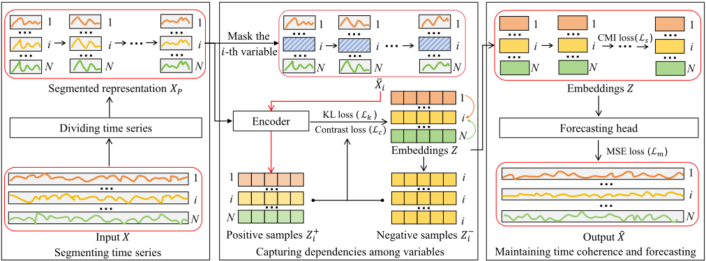
To capture the local intra-correlations in each variable, we divide X into overlapped patches, achieving a segmented representation XP . To reduce redundancy and utilize inter-series correlations when generating embeddings Zi for Xi, we first impose the loss on the encoder to retain useful information for Zi. Then, to capture dependencies among variables, we construct the contrastive learning loss by using positive sample set Z + i and negative sample set Z - i . Thus, the temporal information can be captured from ¯ Xi, which denotes the variables in Xp except Xi. Subsequently, we maximize the CMI between patches within Zi to solve the truncation of the temporal coherence. Additionally, we generate ˆ Xi by Zi and use the Mean Squared Error (MSE) loss between ˆ Xi and its ground truth Yi. Finally, we summarize these steps into an algorithm for MTS forecasting.
4 Methodology
4.1 Framework Overview
We give the framework for MTS forecasting, as shown in Fig.1, including the following components:
- Segmenting time series is proposed to divide time series into overlapped patches, helping the encoder to better capture local intra-series correlations.
- Capturing dependencies among variables is designed and implemented to leverage the CIB principle to identify and capture complex interactions among variables.
- Maintaining time coherence and forecasting is proposed to maintain the intrinsic consistency of MTS by leveraging CMI and then generating forecasting results.
4.2 Conditional Information Bottleneck for Inter-Series Correlation
To capture the dependencies among variables, we employ I(Zi; ¯Xi)(1 ≤ i ≤ N) to quantify the information shared between Zi and ¯Xi, where Zi is generated by qϕ(Zi | Xi) and qϕ(·) denotes the multi-head attention with parameters ϕ.
Maximizing I(Zi; ¯Xi) encourages Zi to capture the dependencies among variables. For this, we adopt the CIB principle centered on I(Zi; ¯Xi), designed to achieve three key objectives: capturing dependencies among variables, minimizing redundancy, and forecasting future observations.
Capturing dependencies among variables. Directly maximizing I(Zi; ¯Xi) for capturing dependencies proves unattainable due to the intricate estimation involved in highdimensional joint distributions. Consequently, we employ the InfoNCE loss [Oord et al., 2018], which establishes a manageable bound to approximate the mutual information:
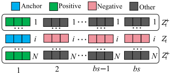
To construct the InfoNCE loss, we first generate the anchor sample set Z anchor i by selecting Zi within the current batch. Then, we generate the positive sample set Z + i by qϕ(Z + i | ¯Xi), which exclusively contains temporal information from other variables, serving as a reference for capturing dependencies among variables. Positive samples Z + ij = {Z + i1 , Z + i2 , . . . , Z + iN } ∈ Z + i (j ̸= i) consist of all variables in Z + i except the i-th variable, which share the same sample index as Z anchor i .
To prevent Zi excessively focusing on temporal information within its own context Xi, the negative sample set Z - i is generated by selecting Zi from each sample within current batch, where Z - il = {Z - i1 , Z - i2 , . . . , Z - ibs } ∈ Z - i within the current batch represents negative samples, and bs denotes batch size. All the samples are selected exclusively from the current batch, shown as Fig.2. Meanwhile, other labels in Fig.2 refer to the unused data points.
Subsequently, we pair Z anchor i with Z + ij to form positive pairs, and Z anchor i with Z - il to form negative pairs. The similarity between positive and negative pairs can be computed using the Cosine similarity function:
where z1 and z2 are the representations of the feature embeddings of two data samples, respectively.
Finally, we impose the inter-series contrastive loss to approximate I(Zi; ¯Xi) by amplifying the similarity of positive pairs and diminishing the similarity of negative pairs at the batch level.
Redundancy minimization. To reduce the forecastingirrelevant information in Zi, we introduce I(Zi; XP ) to quantify the information shared between Zi and XP . This measure is minimized to prompt Zi to concentrate on pertinent temporal data. Given the intractability of directly minimizing I(Zi;XP ), we employ the Kullback-Leibler (KL) divergence [Kullback, 1997] to establish a feasible upper limit for I (Zi; XP ).
To enable the subsequent use of KL divergence, we first express I(Zi; XP ) using variational probability distributions qϕ(Zi; XP ) and qϕ(Zi) as follows:
Without the distributional constraints, Eq. (11) can still result in overfitting and temporal redundancy in Zi, while qϕ(Zi) is still intractable. Thus, we reformulate I(Zi;XP ) by introducing a standard Gaussian distribution p(Zi) ∼ N(0, I ) into Eq. (11).
To further simplify the minimization of I(Zi; XP ) and impose distributional constraints on Zi, we decompose Eq. (12) into two KL divergence terms:
Given the non-negativity property of the KL divergence, the upper limit of Eq. (13) is:
Eq. (14) can be formulated using the KL divergence and minimized to constrict the information capacity of Zi by promoting qϕ(Zi | Xp) to approximate p(Zi). This process aids in reducing redundancy in the encoding of Zi and minimizing I(Zi;XP ). Therefore, we designate Eq. (14) as the redundancy minimization loss, denoted by Lk.
Future observation forecasting. To encourage Zi to contain more information w.r.t. the ground truth Yi, we formulate I(Zi; Yi) to quantify the shared information between Zi and Yi as follows:
Maximizing I(Zi; Yi) promotes the retention of relevant information in Zi for forecasting Yi. To enable a tractable maximization for the mutual information, we assume that Yi is generated by transforming Zi through a linear transformation model with Gaussian noise ϵ.
where ξ denotes the model's parameters.
Assuming that ϵ ∼ N(0, σ2 ) holds, the conditional distribution of Yi given Zi conforms to a Gaussian distribution (i.e., Yi | Zi ∼ N(fξ(Zi), σ2 ), enabling the direct computation of the conditional entropy H(Yi | Zi) as:
where σ2 is the variance of the Gaussian noise and can be formulated as MSE loss.
By substituting Eq. (18) into Eq. (17) and substituting Eq. (17) into Eq. (15), we have
Since H(Yi) is constant, minimizing MSE(Yi, ˆXi) is equivalent to maximizing I(Zi; Yi). Thus, we give the MSE loss Lm to maximize I(Zi; Yi) in a tractable way.
To establish a unified method for the CIB principle, we give three loss components Lm, Lk, and Lc to minimize I(Zi; Yi), I(Zi;Xp), and I(Zi; ¯Xi), respectively. By integrating these objectives, the unified loss function is formulated as:
4.3 Conditional Mutual Information for Intra-Series Correlation
To maintain temporal coherence in MTS, we give the CMIbased principle, which we aim to maximize for each pair of adjacent embedding patches Zik and Zik-1 (1 ≤ k ≤ M) at the data sample level, where M denotes the number of patches and Zik denotes the k-th patch in Zi. These adjacent patches are conditioned on all preceding patches {Zik-2 , . . . , Zi1 }, formulated as:
In order to optimize Eq. (22), we employ the Mutual Information Neural Estimator (MINE) [Belghazi et al., 2018]. MINE establishes a computationally feasible lower bound for I(X; Z) through the dual form of KL divergence, thereby circumventing the direct computation of high-dimensional joint and marginal distributions.
where {Tθ}θ∈Θ denotes the functions parametrized by a neural network, and ˆP means the empirical distribution associated to n i.i.d. samples.
Constructing a computationally feasible lower bound for I (Zik ;Zik-1 | Zik-2 , . . . ,Zi1 ) directly from Eq. (23) poses a challenge. To tackle this issue, we initially reformulate it in terms of the KL divergence.
Expanding upon this representation, we utilize Eq. (23) to establish a lower bound for the CMI. Through parameterizing the CMI distribution with a neural network-based variational function, the resulting computationally manageable lower bound is articulated as
The first term in Eq. (25) signifies the expectation of Tθ within the joint distribution of {Zik ,Zik-1 ,Zik-2 , . . . ,Zi1 }, reflecting the ability of Tθ to capture the true conditional dependencies present in the data. It assigns greater values when Zik and Zik-1 , given {Zik-2 , . . . ,Zi1 }, exhibit stronger correlation. The second term corresponds to the logarithm of the expected value of eTθ under a factorized distribution approximating a scenario, where Zik and Zik-1 are conditionally independent given {Zik-2 , . . . ,Zi1 }. Specifically, we approximate this factorized distribution by shuffling Zik and Zik-1 while keeping {Zik-2 , . . . , Zi1 } fixed to prevent overestimation of the mutual information between Zik and Zik-1 . By computing the difference between these terms, a tractable lower bound on the CMI is derived, which can be optimized w.r.t. Tθ.
In essence, Eq.(25) furnishes a computationally manageable lower bound for the CMI. This bound is employed for every CMI component within Eq.(22) to delineate the loss function Ls, ensuring the temporal coherence of MTS data.
4.4 Training Algorithm
In terms of inter / intra-series correlations, the larger the interseries correlation, the smaller the inter-series loss. Meanwhile, the larger the intra-series correlation, the larger the intra-series loss. To train the forecasting model, we give the total objective as follows:
where Lm is associated with the forecasting task, encouraging the model to accurately forecast future values. Lk focuses on removing irrelevant information. Lc captures the dependencies among variables, and Ls maintains time coherence of MTS. The hyperparameter α1 serves as a regularization coefficient in CIB, balancing the inter-series temporal interactions and preventing overfitting. α2 regulates the strength of time coherence preservation across patches, encouraging the model to capture consistent temporal patterns while controlling its impact on forecasting performance.
Then, we develop the method simultaneously capturing inter and intra-series correlations, summarized in Algorithm 1. The computation of inter-series correlation from line 4 to line 7 takes O(M · d2 + L · d) time, and the computation of intra-series correlation from line 8 to line 13 takes O(M · d) time. Thus, the total time complexity of Algorithm 1 is O(M · d2 + L · d).
5 Experiments
5.1 Experiment Setup
Datasets. We conduct extensive experiments on 9 realworld datasets, as outlined in [Huang et al., 2024], including ETT datasets (ETTh1, ETTh2, ETTm1, ETTm2), Weather, Traffic, Electricity, ILI, and Exchange Rate. In all experiments, we adopt the same train/val/test split ratio of 6:2:2 for ETT datasets and 7:1:2 for others.
Comparison methods. We compare our method with 8 state-of-the-art methods in 5 categories: (a) Transformerbased models: Crossformer [Zhang and Yan, 2023]. Informer [Zhou et al., 2023]. (b) Linear-based models: HDMixer [Huang et al., 2024]. DLinear [Zeng et al., 2023]. (c) CNNbased model: MICN [Wang et al., 2023]. (d) GNN-based models: MSGNet [Cai et al., 2024]. MTGNN [Wu et al., 2020]. (e) IB-based model: LaST [Wang et al., 2022b].
Metrics. We adopt MSE andmean absolute error (MAE) to evaluate the effectiveness of our method.
5.2 Experimental Results
Effectiveness. We compare the MSE and MAE of all models on various datasets, shown in Table 1, where the input sequence length L is set to 96 for Exchange, 60 for ILI, and 336 for others. The lower the indicators, the better the results. In the table, red bold numbers indicate the best performance, while blue indicates the second best. Based on the results, we observe the following:
- (a) Our method achieves superior performance in 67 metrics, matching the SOTA methods in 3 metrics and ranking second in the remaining 2 metrics.
Algorithm 1 CIB-based MTS forecasting
Input: X: historical MTS data
Parameters: P: length of patches, T: total training epochs, lr: learning rate, ϕ: parameters of encoder, θ: parameters of variational bound, ξ: parameters of forecasting head
Output: ˆX: forecasting results
- 1: Divide X into M overlapped patches Xp
- 2: Initialize ϕ, θ, and ξ
- 3: for t = 1 to T do
- 4: Z ← qϕ(Z|XP )
- 5: Calculate Lk by Eq. (14) // Constraint on encoder
- 6: Generate samples Z + i and Z - i
7: Calculate Lc by Eq. (9) // Inter-series correlations
- 8: Ls ← 0
- 9: for k = 3 to M do
- 10: Calculate Iθ(Zik ;Zik-1 |Zik-2 , . . . ,Zi1 )
- 11: Ls ←Ls + Iθ(Zik ;Zik-1 |Zik-2 , . . . ,Zi1 )
- 12: end for
- 13: Ls ←Ls/(M -2) // Constraint on time coherences
- 14: ˆX ← fξ(Z) // Generating forecasting results
- 15: Calculate Lm by Eq. (20) // MSE loss
- 16: L←Lm +α1Lk +α1Lc -α2Ls
- 17: ϕ←ϕ- lr ∗∇L // Updating parameters
- 18: θ ← θ - lr ∗∇L
- 19: ξ ← ξ - lr ∗∇L
- 20: end for
- 21: return ˆX
- (b) Our method outperforms the existing best results by achieving an overall 4.26% reduction in MSE and a 6.12% reduction in MAE. Moreover, our method achieves an overall 60.2% reduction in MSE and 40.5% reduction in MAE when compared to MTGNN.
- (c) Our method outperforms HDMixer, an advanced patchbased model that improves upon PatchTST, achieving overall reductions of 4.26% / 6.12% in MSE / MAE, respectively.
- (d) Our method outperforms the best existing methods without multivariate correlations by achieving an overall 21.4% and 14.3% reduction in MSE and MAE, respectively.
The consistent improvements across all benchmarks underscore the superiority of our method in delivering accurate results across a wide range of datasets and forecasting settings, as reflected in consistently low error metrics.
Ablation studies. We conduct ablation studies on three datasets by removing specific components from our model. The constraints on the encoder, multivariate information interaction, and smooth data transfer are removed by W/O-Lk, W/O-Lc, and W/O-Ls, respectively. From the ablation studies results in Table 2, we can find that:
- (a) When W/O-Lk is applied, MSE increases by up to 5.1% and averages 4.21%, while MAE increases by up to 4.0% with an average of 2.77%.
- (b) When W/O-Lc is performed, the MSE rises a maximum of 5.6% and averaged 3.43%, while the MAE rises a maximum of 3.2% and averaged 1.87%.
- (c) When W/O-Ls is performed, the MSE rises a maximum of 3.04% and averaged 2.01%, while the MAE rises a
| Models | Ours | MSGNet | HDMixer | DLinear | Crossformer | MICN | LaST | Informer | MTGNN | ||||||||||
|---|---|---|---|---|---|---|---|---|---|---|---|---|---|---|---|---|---|---|---|
| Metrics | MSE | MAE | MSE | MAE | MSE | MAE | MSE | MAE | MSE | MAE | MSE | MAE | MSE | MAE | MSE | MAE | MSE | MAE | |
| ILI | 24 36 48 60 | 1.250 1.299 1.220 1.351 | 0.638 0.650 0.644 0.710 | 3.135 3.355 3.588 3.590 | 1.201 1.215 1.306 1.331 | 1.305 1.428 1.233 1.496 | 0.767 0.763 0.798 0.853 | 2.215 1.963 1.673 2.368 | 1.081 0.963 0.854 1.096 | 3.040 3.356 3.441 3.608 | 1.186 1.230 1.223 1.302 | 2.441 2.469 2.430 2.457 | 1.058 1.028 1.037 1.065 | 4.247 4.064 4.559 5.346 | 1.355 1.332 1.440 1.648 | 4.657 4.650 5.004 5.071 | 1.449 1.463 1.542 1.543 | 4.268 4.768 5.333 5.083 | 1.385 1.494 1.592 1.556 |
| Weather | 96 192 336 720 | 0.148 0.194 0.243 0.311 | 0.195 0.237 0.275 0.327 | 0.161 0.204 0.254 0.334 | 0.220 0.257 0.291 0.344 | 0.153 0.200 0.251 0.321 | 0.209 0.249 0.287 0.337 | 0.176 0.220 0.265 0.323 | 0.237 0.282 0.319 0.362 | 0.153 0.197 0.252 0.318 | 0.217 0.269 0.311 0.363 | 0.161 0.220 0.275 0.323 | 0.226 0.283 0.328 0.356 | 0.169 0.197 0.257 0.315 | 0.219 0.238 0.285 0.327 | 0.354 0.419 0.583 0.916 | 0.405 0.434 0.543 0.705 | 0.161 0.206 0.261 0.324 | 0.223 0.278 0.322 0.366 |
| Traffic | 96 192 336 720 | 0.390 0.394 0.418 0.447 | 0.273 0.281 0.287 0.305 | 0.576 0.602 0.621 0.633 | 0.357 0.366 0.370 0.374 | 0.405 0.416 0.428 0.461 | 0.286 0.288 0.297 0.314 | 0.410 0.423 0.436 0.466 | 0.282 0.287 0.296 0.315 | 0.512 0.523 0.530 0.573 | 0.290 0.297 0.300 0.313 | 0.508 0.536 0.525 0.571 | 0.301 0.315 0.310 0.323 | 0.520 0.579 0.616 0.689 | 0.338 0.367 0.419 0.452 | 0.733 0.777 0.776 0.827 | 0.410 0.435 0.434 0.466 | 0.527 0.534 0.540 0.557 | 0.316 0.320 0.335 0.343 |
| Electricity | 96 192 336 720 | 0.130 0.147 0.167 0.201 | 0.221 0.235 0.258 0.285 | 0.143 0.166 0.176 0.252 | 0.252 0.271 0.281 0.367 | 0.137 0.152 0.171 0.212 | 0.241 0.246 0.267 0.296 | 0.140 0.153 0.169 0.203 | 0.237 0.249 0.267 0.301 | 0.187 0.258 0.323 0.404 | 0.283 0.330 0.369 0.423 | 0.159 0.168 0.196 0.203 | 0.267 0.279 0.308 0.312 | 0.161 0.170 0.188 0.223 | 0.257 0.265 0.280 0.309 | 0.304 0.327 0.333 0.351 | 0.393 0.417 0.422 0.427 | 0.198 0.266 0.328 0.422 | 0.294 0.339 0.373 0.410 |
| ETTh1 | 96 192 336 720 | 0.361 0.383 0.385 0.420 | 0.388 0.407 0.409 0.443 | 0.422 0.449 0.461 0.499 | 0.439 0.459 0.466 0.501 | 0.373 0.412 0.392 0.448 | 0.398 0.420 0.417 0.463 | 0.375 0.405 0.439 0.472 | 0.399 0.416 0.443 0.490 | 0.386 0.419 0.440 0.519 | 0.429 0.444 0.461 0.524 | 0.396 0.430 0.433 0.474 | 0.427 0.453 0.458 0.508 | 0.398 0.468 0.566 0.740 | 0.414 0.453 0.512 0.650 | 0.941 1.007 1.038 1.144 | 0.769 0.786 0.784 0.857 | 0.439 0.476 0.736 0.916 | 0.461 0.477 0.643 0.750 |
| ETTh2 | 96 192 336 720 | 0.260 0.314 0.302 0.374 | 0.326 0.365 0.365 0.418 | 0.355 0.407 0.391 0.406 | 0.401 0.432 0.423 0.442 | 0.267 0.317 0.306 0.390 | 0.332 0.367 0.367 0.421 | 0.289 0.383 0.448 0.605 | 0.353 0.418 0.465 0.551 | 0.628 0.703 0.827 1.181 | 0.563 0.624 0.675 0.840 | 0.289 0.409 0.417 0.426 | 0.357 0.438 0.452 0.473 | 0.377 0.619 0.849 0.874 | 0.426 0.639 0.805 0.679 | 1.549 3.792 4.215 3.656 | 0.952 1.542 1.642 1.619 | 0.690 0.745 0.886 1.299 | 0.614 0.662 0.721 0.936 |
| ETTm1 | 96 192 336 720 | 0.289 0.327 0.361 0.413 | 0.337 0.360 0.383 0.417 | 0.303 0.353 0.379 0.429 | 0.360 0.391 0.408 0.437 | 0.291 0.332 0.363 0.424 | 0.341 0.364 0.385 0.417 | 0.299 0.335 0.369 0.425 | 0.343 0.365 0.386 0.421 | 0.316 0.377 0.431 0.600 | 0.373 0.411 0.442 0.547 | 0.314 0.359 0.398 0.459 | 0.360 0.387 0.413 0.464 | 0.323 0.346 0.395 0.493 | 0.360 0.376 0.404 0.470 | 0.626 0.725 1.005 1.133 | 0.560 0.619 0.741 0.845 | 0.428 0.509 0.577 0.713 | 0.446 0.491 0.556 0.729 |
| ETTm2 | 96 192 336 | 0.160 0.213 0.266 | 0.247 0.285 0.321 0.373 | 0.186 0.249 0.301 0.401 | 0.273 0.314 0.347 0.407 | 0.162 0.213 0.275 0.355 | 0.254 0.289 0.331 0.380 | 0.167 0.224 0.281 0.397 | 0.260 0.303 0.342 0.421 | 0.421 0.503 0.611 | 0.461 0.519 0.580 0.750 | 0.178 0.245 0.295 0.389 | 0.273 0.316 0.350 0.406 | 0.174 0.234 0.352 0.911 | 0.265 0.310 0.397 0.671 | 0.355 0.595 1.270 | 0.462 0.586 0.871 | 0.463 0.530 0.449 | 0.503 0.547 0.473 0.836 |
| Exchange | 720 96 192 336 720 | 0.349 0.079 0.164 0.304 0.769 | 0.195 0.288 0.396 0.655 | 0.102 0.195 0.360 0.940 | 0.230 0.317 0.436 0.738 | 0.089 0.173 0.322 0.867 | 0.210 0.297 0.408 0.701 | 0.088 0.176 0.313 0.839 | 0.218 0.315 0.427 0.695 | 0.996 0.188 0.456 0.796 1.367 | 0.365 0.532 0.741 0.943 | 0.102 0.172 0.272 0.714 | 0.235 0.316 0.407 0.658 | 0.108 0.212 0.394 1.398 | 0.236 0.343 0.468 1.102 | 3.001 0.847 1.204 1.672 2.478 | 1.267 0.752 0.895 1.036 1.310 | 1.093 0.208 0.459 0.710 1.323 | 0.381 0.512 0.698 0.912 |
| Datasets | ETTm1 | ILI | Weather | ||||||||||
|---|---|---|---|---|---|---|---|---|---|---|---|---|---|
| Models | Metrics | 96 | 192 | 336 | 720 | 96 | 192 | 336 | 720 | 96 | 192 | 336 | 720 |
| Ours | MSE | 0.289 | 0.327 0.360 | 0.361 0.383 | 0.413 | 1.250 | 1.239 | 1.220 | 1.351 | 0.148 | 0.194 | 0.243 | 0.311 |
| MAE | 0.337 | 0.416 | 0.638 | 0.650 | 0.624 | 0.710 | 0.195 | 0.237 | 0.275 | 0.327 | |||
| W/O-Lk | MSE | 0.294 | 0.333 | 0.368 | 0.431 | 1.326 | 1.360 | 1.261 | 1.376 | 0.156 | 0.198 | 0.259 | 0.325 |
| MAE | 0.341 | 0.362 | 0.386 | 0.419 | 0.648 | 0.689 | 0.674 | 0.718 | 0.200 | 0.237 | 0.289 | 0.341 | |
| W/O-Lc | MSE | 0.291 | 0.331 | 0.366 | 0.423 | 1.394 | 1.322 | 1.252 | 1.378 | 0.153 | 0.199 | 0.250 | 0.320 |
| MAE | 0.339 | 0.363 | 0.385 | 0.420 | 0.658 | 0.668 | 0.669 | 0.712 | 0.199 | 0.240 | 0.280 | 0.331 | |
| W/O-Ls | MSE | 0.293 | 0.333 | 0.373 | 0.420 | 1.307 | 1.301 | 1.248 | 1.358 | 0.152 | 0.198 | 0.249 | 0.321 |
| MAE | 0.340 | 0.365 | 0.386 | 0.418 | 0.644 | 0.666 | 0.671 | 0.715 | 0.202 | 0.239 | 0.278 | 0.331 | |
maximum of 2.8% and averaged 1.6%.
These results demonstrate that each component contributes to the model's performance.
6 Conclusion
Our study introduces a method based on CIB for MTS forecasting, aiming to capture both inter / intra-series correlations effectively. CIB is utilized to capture dependencies among variables within manageable bounds, while CMI is leveraged to ensure temporal coherence through a computationally feasible lower bound. Our approach adeptly captures intricate dependencies in MTS data, thereby improving forecasting accuracy compared to traditional methods.
In forthcoming research, we plan to explore the structural relationships inherent in MTS data and design advanced optimization techniques to better capture temporal and crossvariable dependencies for improved forecasting.
Acknowledgments
This paper was supported by the Joint Key Project of National Natural Science Foundation of China (U23A20298), Key Project of Fundamental Research of Yunnan Province (202401AS070138), and Program of Yunnan Key Laboratory of Intelligent Systems and Computing (202405AV340009).
@inproceedings{ijcai2025p627,
  title     = {Conditional Information Bottleneck-Based Multivariate Time Series Forecasting},
  author    = {Li, Xinhui and Duan, Liang and Yu, Lixing and Yue, Kun and Li, Yuehua},
  booktitle = {Proceedings of the Thirty-Fourth International Joint Conference on
               Artificial Intelligence, {IJCAI-25}},
  publisher = {International Joint Conferences on Artificial Intelligence Organization},
  editor    = {James Kwok},
  pages     = {5634--5642},
  year      = {2025},
  month     = {8},
  note      = {Main Track},
  doi       = {10.24963/ijcai.2025/627},
  url       = {https://doi.org/10.24963/ijcai.2025/627},
}
TY - CPAPER TI - Conditional Information Bottleneck-Based Multivariate Time Series Forecasting AU - Li, Xinhui AU - Duan, Liang AU - Yu, Lixing AU - Yue, Kun AU - Li, Yuehua T2 - Proceedings of the Thirty-Fourth International Joint Conference on Artificial Intelligence, IJCAI-25 PB - International Joint Conferences on Artificial Intelligence Organization PY - 2025 SP - 5634 EP - 5642 DO - 10.24963/ijcai.2025/627 UR - https://doi.org/10.24963/ijcai.2025/627 ER -Copied
Machine-readable versions of this paper, for tools and AI agents:





