
SIFAR: A Simple Faster Accelerated Variance-Reduced Gradient Method
Proceedings of the Thirty-Fourth International Joint Conference on Artificial Intelligence. Main Track. Pages 5662-5670.
https://doi.org/10.24963/ijcai.2025/630
Keywords
- Machine Learning: ML: Supervised Learning
- Machine Learning: ML: Optimization
- Data Mining: DM: Big data and scalability
Abstract
In this paper, we propose a simple faster accelerated gradient method called SIFAR for solving the finite-sum optimization problems. Concretely, we consider both general convex and strongly convex settings: i) For general convex finite-sum problems, SIFAR improves previous state-of-the-art result given by Varag. In particular, for large-scale problems or the convergence error is not very small, SIFAR obtains the first optimal result O(n), matching the lower bound. ii) For strongly convex finite-sum problems, we also show that SIFAR can achieve the optimal convergence rate matching the lower bound. Besides, SIFAR enjoys a simpler loopless algorithmic structure while previous algorithms use double-loop structures. Moreover, we provide a novel dynamic multi-stage convergence analysis, which is the key for improving previous results to the optimal rates. Our new theoretical rates and novel convergence analysis for the fundamental finite-sum problem can directly lead to key improvements for many other related problems, such as distributed/federated/decentralized optimization problems. Finally, the numerical experiments show that SIFAR converges faster than the previous state-of-the-art Varag, validating our theoretical results and confirming the practical superiority of SIFAR.
- [Allen-Zhu and Hazan, 2016] Zeyuan Allen-Zhu and Elad Hazan. Variance reduction for faster non-convex optimiza- tion. In International Conference on Machine Learning, pages 699-707, 2016.
- [Allen-Zhu and Orecchia, 2014] Zeyuan Allen-Zhu and Lorenzo Orecchia. Linear coupling: An ultimate uni- fication of gradient and mirror descent. arXiv preprint arXiv:1407.1537, 2014.
- [Allen-Zhu and Yuan, 2015] Zeyuan Allen-Zhu and Yang Yuan. Improved SVRG for non-strongly-convex or sum-of-non-convex objectives. arXiv preprint arXiv:1506.01972, 2015.
- [Allen-Zhu, 2017] Zeyuan Allen-Zhu. Katyusha: the first di- rect acceleration of stochastic gradient methods. In Pro- ceedings of the 49th Annual ACM SIGACT Symposium on Theory of Computing, pages 1200-1205. ACM, 2017.
- [Bao et al., 2025] Hongyan Bao, Pengwen Chen, Ying Sun, and Zhize Li. EFSkip: A new error feedback with linear speedup for compressed federated learning with arbitrary data heterogeneity. In Proceedings of the AAAI Conference on Artificial Intelligence, volume 39, pages 15489-15497, 2025.
- [Beck and Teboulle, 2009] Amir Beck and Marc Teboulle. A fast iterative shrinkage-thresholding algorithm for lin- ear inverse problems. SIAM journal on imaging sciences, 2(1):183-202, 2009.
- [Chang and Lin, 2011] Chih-Chung Chang and Chih-Jen Lin. LIBSVM: a library for support vector machines. ACM transactions on intelligent systems and technology, 2(3):1-27, 2011.
- [Defazio et al., 2014] Aaron Defazio, Francis Bach, and Si- mon Lacoste-Julien. SAGA: A fast incremental gradient method with support for non-strongly convex composite objectives. In Advances in Neural Information Processing Systems, pages 1646-1654, 2014.
- [Duchi et al., 2010] John C Duchi, Shai Shalev-Shwartz, Yoram Singer, and Ambuj Tewari. Composite objective mirror descent. In Conference on Learning Theory, pages 14-26, 2010.
- [Fang et al., 2018] Cong Fang, Chris Junchi Li, Zhouchen Lin, and Tong Zhang. SPIDER: Near-optimal non-convex optimization via stochastic path-integrated differential es- timator. In Advances in Neural Information Processing Systems, pages 687-697, 2018.
- [Ge et al., 2019] Rong Ge, Zhize Li, Weiyao Wang, and Xi- ang Wang. Stabilized SVRG: Simple variance reduction for nonconvex optimization. In Conference on Learning Theory, pages 1394-1448. PMLR, 2019.
- [Ghadimi and Lan, 2012] Saeed Ghadimi and Guanghui Lan. Optimal stochastic approximation algorithms for strongly convex stochastic composite optimization i: A generic algorithmic framework. SIAM Journal on Opti- mization, 22(4):1469-1492, 2012.
- [Hazan, 2019] Elad Hazan. Introduction to online convex optimization. arXiv preprint arXiv:1909.05207, 2019.
- [Johnson and Zhang, 2013] Rie Johnson and Tong Zhang. Accelerating stochastic gradient descent using predictive variance reduction. In Advances in Neural Information Processing Systems, pages 315-323, 2013.
- [Kovalev et al., 2020] Dmitry Kovalev, Samuel Horváth, and Peter Richtárik. Don't jump through hoops and remove those loops: SVRG and Katyusha are better without the outer loop. In Proceedings of the 31st International Con- ference on Algorithmic Learning Theory, 2020.
- [Lan and Zhou, 2015] Guanghui Lan and Yi Zhou. An op- timal randomized incremental gradient method. arXiv preprint arXiv:1507.02000, 2015.
- [Lan and Zhou, 2018] Guanghui Lan and Yi Zhou. Random gradient extrapolation for distributed and stochastic op- timization. SIAM Journal on Optimization, 28(4):2753- 2782, 2018.
- [Lan et al., 2019] Guanghui Lan, Zhize Li, and Yi Zhou. A unified variance-reduced accelerated gradient method for convex optimization. In Advances in Neural Information Processing Systems, pages 10462-10472, 2019.
- [Lan, 2012] Guanghui Lan. An optimal method for stochas- tic composite optimization. Mathematical Programming, 133(1):365-397, 2012.
- [Le Roux et al., 2012] Nicolas Le Roux, Mark Schmidt, and Francis Bach. A stochastic gradient method with an ex- ponential convergence rate for finite training sets. In Ad- vances in Neural Information Processing Systems, pages 2663-2671, 2012.
- [Lei and Jordan, 2016] Lihua Lei and Michael I Jordan. Less than a single pass: Stochastically controlled stochastic gra- dient method. arXiv preprint arXiv:1609.03261, 2016.
- [Lei et al., 2017] Lihua Lei, Cheng Ju, Jianbo Chen, and Michael I Jordan. Non-convex finite-sum optimization via SCSG methods. In Advances in Neural Information Pro- cessing Systems, pages 2345-2355, 2017.
- [Li and Li, 2018] Zhize Li and Jian Li. A simple proximal stochastic gradient method for nonsmooth nonconvex op- timization. In Advances in Neural Information Processing Systems, pages 5569-5579, 2018.
- [Li and Li, 2020] Zhize Li and Jian Li. A fast Anderson- Chebyshev acceleration for nonlinear optimization. In International Conference on Artificial Intelligence and Statistics, pages 1047-1057. PMLR, 2020.
- [Li and Li, 2022] Zhize Li and Jian Li. Simple and opti- mal stochastic gradient methods for nonsmooth noncon- vex optimization. Journal of Machine Learning Research, 23(239):1-61, 2022.
- [Li and Richtárik, 2020] Zhize Li and Peter Richtárik. A uni- fied analysis of stochastic gradient methods for nonconvex federated optimization. arXiv preprint arXiv:2006.07013, 2020.
- [Li and Richtárik, 2021] Zhize Li and Peter Richtárik. CANITA: Faster rates for distributed convex optimization with communication compression. In Advances in Neu- ral Information Processing Systems, pages 13770-13781, 2021.
- [Li et al., 2020] Zhize Li, Dmitry Kovalev, Xun Qian, and Peter Richtárik. Acceleration for compressed gradient de- scent in distributed and federated optimization. In Inter- national Conference on Machine Learning, pages 5895- 5904. PMLR, 2020.
- [Li et al., 2021a] Zhize Li, Hongyan Bao, Xiangliang Zhang, and Peter Richtárik. PAGE: A simple and optimal probabilistic gradient estimator for nonconvex optimiza- tion. In International Conference on Machine Learning, pages 6286-6295. PMLR, 2021.
- [Li et al., 2021b] Zhize Li, Slavomír Hanzely, and Peter Richtárik. ZeroSARAH: Efficient nonconvex finite-sum optimization with zero full gradient computation. arXiv preprint arXiv:2103.01447, 2021.
- [Li, 2019] Zhize Li. SSRGD: Simple stochastic recursive gradient descent for escaping saddle points. In Advances in Neural Information Processing Systems, pages 1523- 1533, 2019.
- [Lin et al., 2015] Hongzhou Lin, Julien Mairal, and Zaid Harchaoui. A universal catalyst for first-order optimiza- tion. In Advances in Neural Information Processing Sys- tems, pages 3384-3392, 2015.
- [Mairal, 2013] Julien Mairal. Optimization with first-order surrogate functions. In International Conference on Ma- chine Learning, pages 783-791. PMLR, 2013.
- [Mairal, 2015] Julien Mairal. Incremental majorization- minimization optimization with application to large-scale machine learning. SIAM Journal on Optimization, 25(2):829-855, 2015.
- [Nemirovski and Yudin, 1983] Arkadi Nemirovski and David Yudin. Problem complexity and method efficiency in optimization. Wiley-Interscience Series in Discrete Mathematics. John Wiley, XV, 1983.
- [Nemirovski et al., 2009] Arkadi Nemirovski, Anatoli Judit- sky, Guanghui Lan, and Alexander Shapiro. Robust stochastic approximation approach to stochastic program- ming. SIAM Journal on optimization, 19(4):1574-1609, 2009.
- [Nesterov, 1983] Yurii Nesterov. A method for uncon- strained convex minimization problem with the rate of convergence o(1/k 2 ). In Doklady AN USSR, volume 269, pages 543-547, 1983.
- [Nesterov, 2004] Yurii Nesterov. Introductory Lectures on Convex Optimization: A Basic Course. Kluwer, 2004.
- [Nguyen et al., 2017] Lam M Nguyen, Jie Liu, Katya Scheinberg, and Martin Takáč. SARAH: A novel method for machine learning problems using stochastic recursive gradient. In International Conference on Machine Learn- ing, pages 2613-2621, 2017.
- [Pham et al., 2019] Nhan H Pham, Lam M Nguyen, Dzung T Phan, and Quoc Tran-Dinh. ProxSARAH: An efficient al- gorithmic framework for stochastic composite nonconvex optimization. arXiv preprint arXiv:1902.05679, 2019.
- [Reddi et al., 2016a] Sashank J Reddi, Ahmed Hefny, Suvrit Sra, Barnabás Póczos, and Alex Smola. Stochastic vari- ance reduction for nonconvex optimization. In Interna- tional Conference on Machine Learning, pages 314-323, 2016.
- [Reddi et al., 2016b] Sashank J Reddi, Suvrit Sra, Barnabás Póczos, and Alexander J Smola. Proximal stochastic methods for nonsmooth nonconvex finite-sum optimiza- tion. In Advances in Neural Information Processing Sys- tems, pages 1145-1153, 2016.
- [Schmidt et al., 2017] Mark Schmidt, Nicolas Le Roux, and Francis Bach. Minimizing finite sums with the stochas- tic average gradient. Mathematical Programming, 162(1- 2):83-112, 2017.
- [Shalev-Shwartz and Ben-David, 2014] Shai Shalev- Shwartz and Shai Ben-David. Understanding machine learning: from theory to algorithms. Cambridge University Press, 2014.
- [Shalev-Shwartz and Zhang, 2013] Shai Shalev-Shwartz and Tong Zhang. Stochastic dual coordinate ascent methods for regularized loss minimization. Journal of Machine Learning Research, 14(2), 2013.
- [Su et al., 2014] Weijie Su, Stephen P Boyd, and Em- manuel J Candès. A differential equation for modeling Nesterov's accelerated gradient method: Theory and in- sights. In Advances in Neural Information Processing Sys- tems, pages 2510-2518, 2014.
- [Wang et al., 2018] Zhe Wang, Kaiyi Ji, Yi Zhou, Yingbin Liang, and Vahid Tarokh. Spiderboost: A class of faster variance-reduced algorithms for nonconvex optimization. arXiv preprint arXiv:1810.10690, 2018.
- [Woodworth and Srebro, 2016] Blake E Woodworth and Nati Srebro. Tight complexity bounds for optimizing com- posite objectives. In Advances in Neural Information Pro- cessing Systems, pages 3639-3647, 2016.
- [Xiao and Zhang, 2014] Lin Xiao and Tong Zhang. A prox- imal stochastic gradient method with progressive variance reduction. SIAM Journal on Optimization, 24(4):2057- 2075, 2014.
- [Zhao et al., 2021] Haoyu Zhao, Zhize Li, and Peter Richtárik. FedPAGE: A fast local stochastic gradient method for communication-efficient federated learning. arXiv preprint arXiv:2108.04755, 2021.
- [Zhao et al., 2024] Haoyu Zhao, Konstantin Burlachenko, Zhize Li, and Peter Richtárik. Faster rates for compressed federated learning with client-variance reduction. SIAM Journal on Mathematics of Data Science, 6(1):154-175, 2024.
- [Zhou et al., 2018] Dongruo Zhou, Pan Xu, and Quanquan Gu. Stochastic nested variance reduction for nonconvex optimization. In Advances in Neural Information Process- ing Systems, pages 3925-3936, 2018.
References were extracted automatically from the PDF and may contain errors.
Full text extracted automatically from the PDF; figures, tables and equations may differ. The PDF is the version of record.
1 Introduction
In this paper, we consider the fundamental finite-sum problems of the form
where f : Rd → R is a smooth and convex function. We consider two settings in this paper, i) general convex setting
(µ = 0); ii) strongly convex setting (µ > 0), where µ is the strongly convex parameter for f(x), i.e., f(x) - f(y) - ⟨∇f(y), x - y⟩ ≥ µ2 ∥x - y∥2 . Note that the case µ = 0 reduces to the standard convexity. Also note that the strong convexity is only corresponding to the average function f, is not needed for these component functions fis.
Finite-sum problem (1) captures the standard empirical risk minimization (ERM) problems in machine learning [ShalevShwartz and Ben-David, 2014]. There are n data samples and fi denotes the loss associated with i-th data sample, and the goal is to minimize the loss over all data samples. This optimization problem has found a wide range of applications in machine learning, statistical inference, and image processing. In recent years, there has been extensive research in designing gradient-type methods for solving this problem (1). To measure the efficiency of algorithms for solving (1), it is standard to bound the number of stochastic gradient computations for finding a suitable solution. In particular, our goal is to find a point ̂ x ∈ Rd such that E[f(̂ x) - f(x∗ )] ≤ ϵ, where the expectation is with respect to the randomness inherent in the algorithm. We use the term ϵ-approximate solution to refer to such a point ̂ x, and use the term stochastic gradient complexity to describe the convergence result (convergence rate) of algorithms.
Two of the most classical gradient-type algorithms are gradient descent (GD) and stochastic gradient descent (SGD) (e.g., [Nemirovski and Yudin, 1983; Nesterov, 2004; Nemirovski et al., 2009; Duchi et al., 2010; Lan, 2012; Ghadimi and Lan, 2012; Hazan, 2019]). However, GD requires to compute the full gradient over all n data samples for each iteration (xt+1 = xt - η 1n ∑ni=1 ∇fi(xt)) which is inefficient especially for large-scale machine learning problems where n is very large. Although SGD only needs to compute a single stochastic gradient (e.g., ∇fi(x)) for each iteration (xt+1 = xt - η∇fi(xt)), it requires an additional bounded variance assumption for the stochastic gradients (i.e., ∃σ > 0, Ei[∥∇fi(x) - ∇f(x)∥2 ] ≤ σ2 ) since it does not compute the full gradients (∇f(x), i.e., 1n ∑ni=1 ∇fi(x)). More importantly, for strongly convex problems, SGD only obtains a sublinear convergence rate O( σ2 µϵ ) rather than a linear rate O(· log 1ϵ ) achieved by GD.
To remedy the variance term E[∥∇fi(x) - ∇f(x)∥2 ] in SGD, the variance reduction technique has been proposed and it has been widely-used in many algorithms in recent years. In particular, [Le Roux et al., 2012; Schmidt et al., 2017] propose the first variance-reduced algorithm called SAG and show that by incorporating new gradient estimators into SGD one can possibly achieve the linear convergence rate for strongly convex problems. Then this variance reduction direction is followed by many works such as [Shalev-Shwartz and Zhang, 2013; Mairal, 2013; Johnson and Zhang, 2013; Defazio et al., 2014; Mairal, 2015; Nguyen et al., 2017]. Particularly, SAG [Le Roux et al., 2012] uses a biased gradient estimator while SAGA [Defazio et al., 2014] modifies it to an unbiased estimator and provides better convergence results. [Johnson and Zhang, 2013] propose a novel unbiased stochastic variance reduced gradient (SVRG) method which directly incorporates the full gradient term ∇f(x) into SGD. More specifically, each epoch of SVRG starts with the computation of the full gradient ∇f(˜x) at a snapshot point ˜x ∈ Rn and then runs SGD for a fixed number of steps using the modified stochastic gradient estimator
i.e., xt+1 = xt - η˜∇t, where i is randomly picked from {1, 2, . . . , n}. In particular, if each full gradient ∇f(˜x) (which requires n stochastic gradient computations) at the snapshot point ˜x is reused for n iterations (i.e., ˜x is changed after every n iterations), then the amortized stochastic gradient computations for each iteration is the same as SGD. Note that E[˜∇t] = ∇f(xt) is an unbiased estimator, and its variance E[∥˜∇t - ∇f(xt)∥2 ] ≤ 4L(f(xt) - f(x∗ ) + f(˜x)-f(x∗ )) is reduced as the algorithm converges xt, ˜x → x∗ , while the variance term is uncontrollable for plain SGD where ˜∇t = ∇fi(xt). [Johnson and Zhang, 2013] also show that SVRG obtains the linear convergence O((n + Lµ ) log 1ϵ ) which can be better than the sublinear convergence rate O( σ2 µϵ ) of plain SGD, for strongly convex problems. The SVRG gradient estimator (2) is adopted in many algorithms (e.g., [Xiao and Zhang, 2014; Allen-Zhu and Yuan, 2015; Lei and Jordan, 2016; Allen-Zhu and Hazan, 2016; Reddi et al., 2016a; Reddi et al., 2016b; Lei et al., 2017; Li and Li, 2018; Zhou et al., 2018; Ge et al., 2019; Kovalev et al., 2020; Li and Li, 2022]) and also is used in our SIFAR.
The aforementioned variance-reduced methods are not accelerated and hence they do not achieve the optimal convergence rates for convex finite-sum problem (1). See the nonaccelerated variance-reduced algorithms listed in the first part of Table 1, i.e., SAG, SVRG, SAGA and SVRG ++ , they do not achieve the accelerated rates, i.e., Lµ vs. √ Lµ (strongly
convex case) and Lϵ vs. √ Lϵ (general convex case). Note
that we do not list the SCSG [Lei and Jordan, 2016] and SARAH [Nguyen et al., 2017] in Table 1 since SCSG requires an additional bounded variance assumption (without this assumption, its result is the same as SVRG and SAGA) and SARAH uses E[∥∇f (̂ x)∥2 ] ≤ ϵ as the convergence criterion which can not be directly converted to E[f(̂ x) - f(x∗ )] ≤ ϵ. SARAH is usually used for solving nonconvex problems where the convergence criterion is typically the norm of gradient (e.g., [Fang et al., 2018; Wang et al., 2018; Pham et al., 2019; Li, 2019; Li et al., 2021b; Li et al., 2021a]). Also both SCSG and SARAH are non-accelerated methods and thus do not achieve the optimal convergence results. Therefore, much recent research effort has been devoted to the design of accelerated gradient methods (e.g., [Nesterov, 2004; Beck and Teboulle, 2009; Lan, 2012; Allen-Zhu and Orecchia, 2014; Su et al., 2014; Lin et al., 2015; Allen-Zhu, 2017; Lan and Zhou, 2018; Lan et al., 2019; Li and Li, 2020; Li et al., 2020]). As shown in Table 1, for strongly convex finite-sum problems, existing accelerated methods such as RPDG [Lan and Zhou, 2015], Katyusha [Allen-Zhu, 2017], Varag [Lan et al., 2019] and our SIFAR are optimal since their convergence results are O((n + √ nL µ ) log 1ϵ ) matching the lower bound Ω((n + √ nL µ ) log 1ϵ ) given by [Lan and Zhou, 2015].
However, for general (non-strongly) convex finite-sum problems, all previous accelerated methods do not achieve the optimal convergence result. In particular, Varag [Lan et al., 2019] obtains the current best result O(nmin{log 1ϵ , log n}+ √ nL ϵ ), while the lower bound in this general convex case is Ω(n + √ nL ϵ ) provided by [Woodworth and Srebro, 2016]. More importantly, for large-scale problems where the number of data samples n is very large, or the convergence error ϵ is not very small, then the convergence result of Varag is O(n log 1ϵ ) which is not optimal since the lower bound is Ω(n) (see Table 2). Note that the case of large-scale problems or the case of moderate convergence error often exists in machine learning applications. We show that our SIFAR takes an important step towards the ultimate limit of accelerated methods and it is the first algorithm to achieve the optimal convergence rate O(n) in this case matching the lower bound Ω(n). See Tables 1 and 2 for more details.
2 Our Contributions
In this paper, we mainly focus on further improving the convergence result in order to close the gap between the upper and lower bound. We propose a novel loopless accelerated variance-reduced gradient method, called SIFAR (Algorithm 1), for solving both general convex and strongly convex finite-sum problems given in the form of (1). Tables 1 and 2 summarize the convergence results of previous algorithms and SIFAR.
Now, we highlight the following results achieved by SIFAR:
- For general convex problems, SIFAR obtains the rate O(nmin {1 + log 1 ϵ√n , log √n} + √ nL ϵ ) for finding an ϵ-approximate solution of problem (1), which improves previous best result O(nmin{log 1ϵ , logn} + √ nL ϵ ) given by Varag [Lan et al., 2019] (see the 'general convex' column of Table 1). Moreover, for a very wide range of ϵ, i.e., ϵ ∈ (0, L n log2 √n ]∪[ 1 √n , +∞), or the number of data samples n ∈ (0, L ϵ log2 √n ] ∪ [ 1 ϵ2 , +∞), SIFAR can exactly achieve the
| Algorithms | µ-strongly convex | General convex | Simple (Loopless) |
|---|---|---|---|
| GD | O ( nL µ log 1ϵ ) | O ( nL ϵ ) | Yes |
| Nesterov's AGD [Nesterov, 1983; Nesterov, 2004] | O (n√ Lµ log 1ϵ ) | O (n√ Lϵ ) | Yes |
| SAG [Le Roux et al., 2012] | O((n+n2 ⌊ L nµ ⌋) log 1ϵ ) | - | Yes |
| SVRG [Johnson and Zhang, 2013] | O ((n+ Lµ ) log 1ϵ ) | - | No |
| SAGA [Defazio et al., 2014] | O ((n + Lµ ) log 1ϵ ) | O ( n+L ϵ ) | Yes |
| SVRG ++ [Allen-Zhu and Yuan, 2015] | - | O (n log 1ϵ + Lϵ ) | No |
| RPDG [Lan and Zhou, 2015] | O ((n+ √ nL µ ) log 1ϵ ) | O ((n + √ nL ϵ ) log 1ϵ ) 1 | Yes |
| Catalyst [Lin et al., 2015] | O ((n + √ nL µ ) log 1ϵ ) 1 | O ((n + √ nL ϵ ) log2 1ϵ ) 1 | No |
| Katyusha [Allen-Zhu, 2017] | O ((n + √ nL µ ) log 1ϵ ) | O (n log 1ϵ + √ nL ϵ ) 1 | No |
| Katyusha ns [Allen-Zhu, 2017] | - | O ( n √ϵ + √ nL ϵ ) | No |
| Varag [Lan et al., 2019] | O ((n + √ nL µ ) log 1ϵ ) | O(nmin { log 1ϵ , logn} + √ nL ϵ ) | No |
| SIFAR (this paper) | O ((n + √ nL µ ) log 1ϵ ) | O(nmin {1+ log 1 ϵ√n , log √n} + √ nL ϵ ) 2 | Yes |
| Lower bound | Ω ((n + √ nL µ ) log 1ϵ ) [Lan and Zhou, 2015] | Ω (n + √ nL ϵ ) [Woodworth and Srebro, 2016] | - |
| Algorithms | The convergence error (E[f(̂ x) - f(x∗ )] ≤ ϵ): large ϵ -→ small ϵ (or the number of data samples: large n -→ small n) | |||
|---|---|---|---|---|
| ϵ ≥ 1 √n | 1 √n > ϵ ≥ 1n | 1n > ϵ ≥ L n log2 √n | L n log2 √n > ϵ | |
| Katyusha ns [Allen-Zhu, 2017] | O ( n √ϵ ) | O ( n √ϵ ) | O ( n √ϵ ) | O( n √ϵ + √ nL ϵ ) |
| Varag [Lan et al., 2019] | O (n log 1ϵ ) | O (n log 1ϵ ) | O (n log n) | O(√ nL ϵ ) |
| SIFAR (this paper) 1 | O(n) | O(n(1+ log 1 ϵ√n )) | O(n log √n) | O(√ nL ϵ ) |
| Lower bound [Woodworth and Srebro, 2016] | Ω(n) | Ω (n) | Ω(n√ L ϵn ) | Ω (√ nL ϵ ) |
Table 2: Direct accelerated stochastic algorithms for general convex setting with respect to ϵ
optimal convergence result O(n+ √ nL ϵ ) matching the lower
2016] (see Table 1 and its Footnote 2).
- In particular, we would like to point out that none of previous algorithms with/without acceleration can obtain the optimal result O(n) for finite-sum problems (1) where the number of data samples is very large or the convergence error is not very small, SIFAR is the first algorithm that achieves the optimal result O(n) for these typical machine learning problems (see the second column of Table 2 and its Remark).
- We also note that SIFAR is the first loopless direct accelerated stochastic algorithm for solving general convex finitesum problems, while previous accelerated stochastic algorithms use indirect approaches (RPDG, Catalyst, Katyusha) and/or use inconvenient double-loop algorithmic structures (Katyusha ns , Varag) (see Table 1). Moreover, by exploiting the loopless structure of SIFAR, we provide a novel dynamic multi-stage convergence analysis which is the key for improving previous results to the optimal rates.
- For strongly convex finite-sum problems (i.e., under strong convexity Assumption 2), we also prove that SIFAR achieves the optimal convergence rate O((n + √ nL µ ) log 1ϵ ) matching the lower bound Ω((n+ √ nL µ ) log 1ϵ ) provided by
[Lan and Zhou, 2015] (see Table 1).
- Moreover, the convergence guarantee of SIFAR is the last iterate convergence, i.e., guarantee for wT (see Corollaries 1 and 2) unlike previous average iterates convergence, i.e., guarantee for ¯wT = 1 T ∑T -1 t=0 qtwt for some distribution q.
- Finally, the numerical experiments show that SIFAR converges faster than the previous state-of-the-art Varag [Lan et al., 2019], validating our theoretical results and confirming the practical superiority of SIFAR.
3 Preliminaries
Notation: Let [n] denote the set {1, 2, · · · , n} and ∥·∥ denote the Euclidean norm for a vector and the spectral norm for a matrix. Let ⟨u, v⟩ denote the inner product of two vectors u and v. We use O(·) and Ω(·) to hide the absolute constant. We will write x∗ := argminx∈Rd f(x).
For convex problems, one typically uses the function value gap as the convergence criterion.
Definition 1. A point ̂ x is called an ϵ-approximate solution for problem (1) if E[f(̂ x) - f (x∗ )] ≤ ϵ.
To show the convergence results, we assume the following standard smoothness assumption for the component functions fis in (1).
Assumption 1 (L-smoothness). Functions fi : Rd → R are convex and L-smooth such that
for some L ≥ 0 and all i ∈ [n].
It is easy to see that f(x) = 1n ∑ni=1 fi(x) is also Lsmooth under Assumption 1.
Algorithm 1 SIFAR: SImple Faster Accelerated varianceReduced gradient
Input: initial point x0, parameters {pt}, {θt}, {ηt}, {αt}
- 1: w0 = ¯x0 = x0 = x0
- 2: for t = 0, 1, 2, . . . , T -1 do
- 3: xt = θtxt + (1 - θt)wt
- 4: Randomly pick i ∈ {1, 2, . . . , n}
- 5: ˜∇t =∇fi(xt ) -∇fi(wt) +∇f(wt)
- 6: xt+1 = 1 1+µηt (xt + µηtxt ) - ηt αt ˜∇t
- 7: ¯xt+1 = θtxt+1 + (1 - θt)wt
- 8: wt+1 = {¯xt+1 with probability pt wt with probability 1-pt
9: end for
Output: wT
For considering the strongly convex setting, we assume the following Assumption 2.
Assumption 2 (µ-strong convexity). A function f : Rd →R is µ-strongly convex such that
for some µ ≥ 0.
Note that the strong convexity is only corresponding to the average function f in (1), is not needed for the component functions fis.
4 SIFARAlgorithm
In this section, we describe the simple SIFAR method in Algorithm 1. SIFAR uses the SVRG gradient estimator (2) (see Line 5 of Algorithm 1) and two interpolation steps (momentum) (see Line 3 and Line 7 of Algorithm 1). Line 6 of Algorithm 1 is a gradient update step.
Although previous accelerated stochastic algorithms such as Katyusha/Katyusha ns [Allen-Zhu, 2017] and Varag [Lan et al., 2019] also adopt the SVRG gradient estimator combined with momentum steps, SIFAR enjoys a simpler loopless algorithmic structure. Note that the previous loopless SVRG/Katyusha algorithms provided in [Kovalev et al., 2020] only solve the strongly convex case (µ > 0). Here, our loopless algorithm SIFAR can deal with both general convex (µ = 0) and strongly convex (µ > 0) problems, and the SIFAR algorithm itself is also different and more concise than the loopless algorithms in [Kovalev et al., 2020]. Moreover, for general convex problems (µ = 0), SIFAR provides a new state-of-the-art convergence result which improves all previous results.
In each iteration t, the stochastic gradient estimator ˜∇t of SIFAR (Line 5 of Algorithm 1) uses the gradient information of only one randomly sampled function fi. Note that for the last term ∇f(wt), it reuses previous ∇f(wt-1) with probability 1 - pt-1 or needs to compute the full gradient ∇f(¯xt) with probability pt-1 (see Line 8 of Algorithm 1). Thus we know that SIFAR uses (n + 2)pt-1 + 2(1 - pt-1) stochastic gradients in expectation for iteration t. In particular, if pt ≡ 1n , then SIFAR only uses constant stochastic gradients for each iteration which maintains the same computational cost as SGD. The snapshot point wt is updated in the last Line 8 of Algorithm 1, it is a probabilistic step which is the key part for removing double-loop structures to obtain a simple loopless algorithm, similar to [Kovalev et al., 2020; Li et al., 2021a]. However, we propose a new dynamic multistage convergence analysis which uses a dynamic control of the probability {pt} in Line 8, unlike directly fixing it to a constant pt ≡ p as in [Kovalev et al., 2020]. To the best of our knowledge, this is the first time that a loopless algorithm uses a dynamic change of {pt}.
5 Convergence Results for SIFAR
In this section, we present two main convergence theorems of SIFAR (Algorithm 1) for solving finite-sum problems (1), i.e., Theorem 1 (general convex setting in Section 5.1) and Theorem 2 (strongly convex setting in Section 5.2). Subsequently, we formulate two Corollaries 1-2 from Theorems 12 for providing the detailed convergence results. The detailed proofs for Theorems 1-2 and Corollaries 1-2 are deferred to the appendix.
5.1 General convex setting
In this section, we provide the main convergence theorem of SIFAR for general convex problems and then obtain a corollary for providing the detailed convergence result. Note that if we fix the probability pt in Line 8 of Algorithm 1 to a constant p, then the update of wt follows from a geometric distribution Geom(p). For a geometric distribution N ∼ Geom(p), i.e., N = k with probability (1 - p)k p for k = 0, 1, 2, . . . (after k failures until the first success), we know that E[N] = 1-p p . In the first stage of SIFAR, we indeed use constant probability pt ≡ p = 1 n+1 . Let t1 be the first time such that w changes to ¯x, i.e., wt1+1 = ¯xt1+1 and wt1 = wt1-1 = · · · = w0. Thus t1 ∼ Geom(p) and E[t1] = n. Note that this first stage where we fix pt ≡ p is similar to loopless SVRG [Kovalev et al., 2020], SCSG [Lei and Jordan, 2016] and PAGE [Li et al., 2021a]. The difference is that our SIFAR will use a dynamic change of pt after the first stage, while previous algorithms always keep fixing the probability pt ≡ p.
Theorem 1 (General convex case). Suppose that Assumption 1 holds. For 0 ≤ t ≤ t1, let pt ≡ 1 n+1 , θt ≡ 1 - 1 2√n , ηt ≤ 1 L(1+1/(1-θt)) and αt = θt. For t > t1, let pt = max{ 4 t-t1+3√n , 4 n+3 }, θt = 2 pt(t-t1+3√n) , ηt ≤ 1 3L and αt = θt. Then the following equation holds for SIFAR (Algorithm 1) for any iteration t > t1 + 1:
According to Theorem 1, we can obtain a detailed convergence result in the following Corollary 1.
Corollary 1 (General convex case). Suppose that Assumption 1 holds. Choose the parameters {pt}, {θt}, {ηt}, {αt} as stated in Theorem 1. Then SIFAR (Algorithm 1) can find an ϵ-approximate solution for problem (1) such that
within T iterations, where
and the number of stochastic gradient computations can be bounded by
Remark: From the choice of probability {pt} in Theorem 1, we know that there are three stages of SIFAR: i) the first stage pt ≡ 1 n+1 for 0 ≤ t ≤ t1; ii) the second stage pt = 4 t-t1+3√n for t1 < t ≤ t1 +n+3-3√n; iii) the third stage pt ≡ 4 n+3 for t > t1 + n + 3 - 3√n. This novel multi-stage convergence analysis is key part for the improvement of SIFAR. Roughly speaking, the number of stochastic gradient computations in the first stage is #grad = O(n), in the second stage is #grad = O(nmin { log 1 ϵ√n , log √n}), and in the third stage is #grad = O(√ nL ϵ ). Note that the guarantee of SIFAR is the last iterate convergence unlike previous average iterates convergence. Also note that all parameter settings {pt}, {θt}, {ηt}, {αt} of SIFAR in Theorem 1 do not require the value of ϵ in advance. The convergence rate of SIFAR will automatically switch to different results as stated in Table 2.
5.2 Strongly convex setting
In this section, we provide the main convergence theorem of SIFAR for strongly convex problems (µ > 0 in Assumption 2) and then obtain a corollary for providing the detailed convergence result.
Theorem 2 (Strongly convex case). Suppose that Assumptions 1 and 2 hold. For any t ≥ 0, let pt ≡ p, θt ≡ θ = 1 2 min{1, √ µ pL }, ηt ≤ 1 Lθt(1+1/(1-θt)) and αt = 1 + µηt. Then the following equation holds for SIFAR (Algorithm 1) for any iteration t ≥ 0:
Similarly, according to Theorem 2, we can obtain a detailed convergence result in the following Corollary 2.
Corollary 2 (Strongly convex case). Suppose that Assumptions 1 and 2 hold. Choose the parameters {pt}, {θt}, {ηt}, {αt} as stated in Theorem 2. Then SIFAR (Algorithm 1) can find an ϵ-approximate solution for problem (1) such that
within T iterations, where
Moreover, by choosing p = 1n and recalling that θ = 12 min{1, √ µ pL }, the number of stochastic gradient computations can be bounded by
Remark: In this strongly convex case, the parameter setting of SIFAR in Theorem 2 is simpler than the general convex case in Theorem 1. Here, the choice of probability {pt} can be fixed to a constant p and {θt} also can be chosen as a constant θ. Then according to Theorem 2, we know that {ηt} and {αt} also reduce to constant values. Thus there is only one stage in this strongly convex case rather than three stages in previous general convex case. Also here the function value decreases in an exponential rate, i.e., E[Φt] ≤ (1 - 4pθ 5 )tΦ0 (see (5) in Theorem 2). It is easy to see that the number of iterations T can be bounded by O(· log 1ϵ ) for finding an ϵ-approximate solution E[f(wT ) - f(x∗ )] ≤ ϵ. Then, by choosing p = 1n (thus each iteration only computes constant stochastic gradients in expectation), the number of total stochastic gradient computations can be bounded by #grad = O( max {n, √ nL µ } log 1ϵ ). This convergence result is optimal which matches the lower bound Ω((n + √ nL µ ) log 1ϵ ) given by [Lan and Zhou, 2015] (see Table 1). Note that all parameter settings {pt}, {θt}, {ηt}, {αt} of SIFAR in Theorem 2 also do not require the value of ϵ in advance.
5.3 Proof sketch for general convex case (Theorem 1)
Now, we provide the proof sketch of Theorem 1. As we discussed in the Remark at the end of Section 5.1, we know that there are three stages of SIFAR. First, we provide a key lemma for the first stage.
Lemma 1. Suppose Assumption 1 holds. For 0 ≤ t ≤ t1, let pt ≡ p, θt ≡ θ, ηt ≤ 1 L(1+1/(1-θt)) and αt = θt. Then the following equation holds for SIFAR (Algorithm 1):
E[f (wt1+1) - f (x∗ )]
According to the update formula of wt in the Line 8 of Algorithm 1, we know that E[t1] = 1-p p . Thus if we let pt ≡ p = 1 n+1 in the first stage of SIFAR (i.e., for 0 ≤ t ≤ t1), then E[t1] = n. The choice of parameters in Lemma 1 with p = 1 n+1 is the same as the first stage of Theorem 1.
After the first stage, for any iteration t > t1, we provide the following technical lemma which describes the change of function value between two adjacent iterations.
Lemma 2. Suppose Assumption 1 holds. Choose stepsize ηt ≤ 1 L(1+1/(1-θt)) and αt = θt for any t ≥ 0. Then the following equation holds for SIFAR (Algorithm 1) for any iteration t ≥ 0:
According to (7), in order to get a recursion formula, we need to show that(1 - ptθt)ηt
by further choosing appropriate parameters {pt} and {θt}. In particular, choosing pt = max{ 4 t-t1+3√n , 4 n+3 } and θt = 2 pt(t-t1+3√n) for t > t1 (same as in Theorem 1) can satisfy (8) for any t > t1 + 1. Combining this choice of {pt} and {θt} with Lemma 2 and summing up from iteration t1 + 1 to t, we obtain the following Lemma 3.
Lemma 3. Suppose Assumption 1 holds. For t > t1, let pt = max{ 4 t-t1+3√n , 4 n+3 }, θt = 2 pt(t-t1+3√n) , ηt ≤ 1 3L and αt = θt. Then the following equation holds for SIFAR (Algorithm 1) for any iteration t > t1 + 1:
Also note that we can bound the term f(x0) - f(x∗ ) in (6) as f(x0) - f(x∗ ) ≤ L2 ∥x0 - x ∗ ∥2 according to the L-smoothness of f (Assumption 1). Now, we combine Lemma 1 and Lemma 3 to finish the proof for the main Theorem 1, i.e., by plugging (6) into (9) and plugging in the value of parameters, we can obtain, for any iteration t > t1 + 1,
6 Experiments
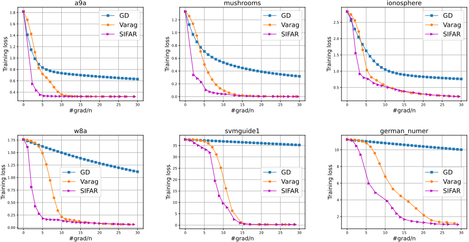
In this section, we present the numerical experiments of SIFAR (Algorithm 1) compared with previous state-of-the-art Varag [Lan et al., 2019]. We also present the standard gradient descent (GD) as a benchmark for demonstrating the performance of these algorithms. The theoretical convergence results of these algorithms can be found in Table 1.
In the experiments, we consider the following logistic regression problem:
where {ai, bi}ni=1 ∈ Rd × {±1} are data samples. All datasets used in our experiments are downloaded from LIBSVM [Chang and Lin, 2011]. We also point out that we directly use the parameter settings according to the theoretical convergence theorems or corollaries of these algorithms, i.e., we do not tune any hyperparameters. Note that for the logistic function in (10), one can precompute the smoothness parameter L satisfying Assumption 1, i.e., L ≤ 1/4 if the data samples are normalized. Given the parameter L, we are ready to set all other hyperparameters for GD (see Corollary 2.1.2 in [Nesterov, 2004]), for Varag (see Theorem 1 in [Lan et al., 2019]) and for SIFAR (see our Theorem 1). Note that all of these three algorithms only require L for setting their (hyper)parameters.
In Figure 1, the x-axis and y-axis represent the number of data passes (i.e., we compute n stochastic gradients for each data pass) and the training loss, respectively. The numerical results presented in Figure 1 are conducted on different datasets. Each plot corresponds to one dataset (six datasets in total). The experimental results show that SIFAR indeed converges faster than Varag [Lan et al., 2019] in the earlier stage (moderate convergence error), validating our theoretical results (see the second column of Table 2 and its Remark). More importantly, SIFAR is the first accelerated algorithm which can obtain the optimal convergence result O(n) in this range. Besides, SIFAR also enjoys a simpler loopless algorithmic structure while Varag uses an double-loop structure.
7 Conclusion
In this paper, we propose a faster loopless accelerated variance-reduced gradient method SIFAR, for solving both general convex and strongly convex finite-sum problems. The proposed SIFAR takes an important step towards the ultimate limit of accelerated methods to close the gap between the upper and lower bound. In particular, SIFAR achieves the first optimal convergence rate O(n) matching the lower bound Ω(n) for large-scale general convex problems. Besides, it also achieves the optimal convergence rate O((n + √ nL µ ) log 1ϵ ) matching the lower bound Ω((n + √ nL µ ) log 1ϵ ) for strongly convex problems. Moreover, we provide a novel dynamic multi-stage convergence analysis utilizing the simpler loopless algorithmic structure, which is the key for improving previous results to the optimal rates. Numerical experiments validate our theoretical results and confirm the practical superiority of SIFAR. Our new theoretical rates and convergence analysis can also lead to key improvements for other related distributed and federated optimization problems, e.g., [Li and Richt´arik, 2020; Li and Richt´arik, 2021; Zhao et al., 2021; Zhao et al., 2024; Bao et al., 2025].
Acknowledgments
This research was supported by the Singapore Ministry of Education (MOE) Academic Research Fund (AcRF) Tier 1 grant.
@inproceedings{ijcai2025p630,
  title     = {SIFAR: A Simple Faster Accelerated Variance-Reduced Gradient Method},
  author    = {Li, Zhize},
  booktitle = {Proceedings of the Thirty-Fourth International Joint Conference on
               Artificial Intelligence, {IJCAI-25}},
  publisher = {International Joint Conferences on Artificial Intelligence Organization},
  editor    = {James Kwok},
  pages     = {5662--5670},
  year      = {2025},
  month     = {8},
  note      = {Main Track},
  doi       = {10.24963/ijcai.2025/630},
  url       = {https://doi.org/10.24963/ijcai.2025/630},
}
TY - CPAPER TI - SIFAR: A Simple Faster Accelerated Variance-Reduced Gradient Method AU - Li, Zhize T2 - Proceedings of the Thirty-Fourth International Joint Conference on Artificial Intelligence, IJCAI-25 PB - International Joint Conferences on Artificial Intelligence Organization PY - 2025 SP - 5662 EP - 5670 DO - 10.24963/ijcai.2025/630 UR - https://doi.org/10.24963/ijcai.2025/630 ER -Copied
Machine-readable versions of this paper, for tools and AI agents:





