
CFDONEval: A Comprehensive Evaluation of Operator-Learning Neural Network Models for Computational Fluid Dynamics
Proceedings of the Thirty-Fourth International Joint Conference on Artificial Intelligence. Main Track. Pages 5752-5760.
https://doi.org/10.24963/ijcai.2025/640
Keywords
- Machine Learning: ML: Applications
- Machine Learning: ML: Evaluation
- Multidisciplinary Topics and Applications: MTA: Physical sciences
Abstract
In this paper, we introduce CFDONEval, a comprehensive evaluation of 12 operator-learning-based neural network (ON) models to simulate 7 benchmark fluid dynamics problems. These problems cover a range of 2D scenarios, including Darcy flow, two-phase flow, Taylor-Green vortex, lid-driven cavity flow, tube flow, circular cylinder flow, and 3D periodic hill flow. For a rigorous evaluation, we establish 22 fluid dynamics datasets for these benchmark problems, 18 of which are newly generated using traditional numerical methods, such as the finite element method. Our evaluation tackles 5 key challenges: multiscale phenomena, convection dominance, long-term predictions, multiphase flows, and unstructured meshes over complex geometries. We assess computational accuracy, efficiency, and flow field visualization, offering valuable insights into the application of ON models in fluid dynamics research. Our findings show that attention-based models perform well in handling almost all challenges; models with a U-shaped structure excel in handling multiscale problems; and the NU-FNO model demonstrates the smallest relative error in L2 norm when processing nonuniform grid data. The related code, dataset, and appendix are publicly available at: https://github.com/Sysuzqs/CFDNNEval.
- [Alleborn et al., 1999] N. Alleborn, H. Raszillier, and F. Durst. Lid-driven cavity with heat and mass trans- port. International Journal of Heat and Mass Transfer, 42(5):833-853, 1999.
- [Almeida et al., 1993] G.P. Almeida, D.F.G. Durão, and M.V. Heitor. Wake flows behind two-dimensional model hills. Experimental Thermal and Fluid Science, 7(1):87- 101, 1993.
- [Anonymous, 2024] Anonymous. MPFBench: A large scale dataset for sciML of multi-phase-flows: Droplet and bub- ble dynamics. In Submitted to The Thirteenth Interna- tional Conference on Learning Representations, 2024. un- der review. [Brandstetter et al., 2022]
- J. Brandstetter, D. E. Worrall, and M. Welling. Message passing neural PDE solvers. In Inter- national Conference on Learning Representations, 2022.
- [Cao, 2021] S. Cao. Choose a transformer: Fourier or Galerkin. In Advances in Neural Information Processing Systems (NeurIPS 2021), volume 34, 2021.
- [COM, 2023] COMSOL Multiphysics ® v. 6.2, Stockholm, Sweden. AC/DC Module User's Guide, 2023.
- [Feng, 2006] X. Feng. Fully discrete finite element approxi- mations of the Navier-Stokes-Cahn-Hilliard diffuse inter- face model for two-phase fluid flows. SIAM Journal on Numerical Analysis, 44(3):1049-1072, 2006.
- [Gal and Grasselli, 2010] C. G. Gal and M. Grasselli. Asymptotic behavior of a Cahn-Hilliard-Navier-Stokes system in 2D. Annales de l'I.H.P. Analyse non linéaire, 27(1):401-436, 2010.
- [Guo et al., 2016] X. Guo, W. Li, and F. Iorio. Convolutional neural networks for steady flow approximation. In Pro- ceedings of the 22nd ACM SIGKDD International Con- ference on Knowledge Discovery and Data Mining, KDD '16, page 481-490, New York, NY, USA, 2016. Associa- tion for Computing Machinery.
- [Gupta and Brandstetter, 2022] J. K. Gupta and J. Brandstet- ter. Towards multi-spatiotemporal-scale generalized pde modeling. arXiv preprint arXiv:2209.15616, 2022.
- [Hao et al., 2023] Z. Hao, Z. Wang, H. Su, C. Ying, Y. Dong, S. Liu, Z. Cheng, J. Song, and J. Zhu. GNOT: A general neural operator transformer for operator learning. In An- dreas Krause, Emma Brunskill, Kyunghyun Cho, Barbara Engelhardt, Sivan Sabato, and Jonathan Scarlett, editors, Proceedings of the 40th International Conference on Ma- chine Learning, volume 202 of Proceedings of Machine Learning Research, pages 12556-12569. PMLR, 23-29 Jul 2023.
- [Hassan et al., 2023] S. M. S. Hassan, A. Feeney, A. Dhruv, J. Kim, Y. Suh, J. Ryu, Y. Won, and A. Chandramowlish- waran. BubbleML: A multiphase multiphysics dataset and benchmarks for machine learning. In Thirty-seventh Conference on Neural Information Processing Systems Datasets and Benchmarks Track, 2023.
- [Kochkov et al., 2021] D. Kochkov, J. A. Smith, A. Alieva, Q. Wang, M. P. Brenner, and S. Hoyer. Ma- chine learning-accelerated computational fluid dynam- ics. Proceedings of the National Academy of Sciences, 118(21):e2101784118, 2021.
- [Lesieur, 2008] M. Lesieur. Turbulence in Fluids. Fluid Me- chanics and Its Applications. Springer Netherlands, 2008.
- [Li et al., 2020] Z. Li, N. Kovachki, K. Azizzadenesheli, B. Liu, K. Bhattacharya, A. Stuart, and A. Anandkumar. Fourier neural operator for parametric partial differential equations. arXiv preprint arXiv:2010.08895, 2020.
- [Li et al., 2023] Z. Li, K. Meidani, and A. Farimani. Trans- former for partial differential equations' operator learning. Transactions on Machine Learning Research, 2023.
- [Liu et al., 2023] S. Liu, Z. Hao, C. Ying, H. Su, Z. Cheng, and J. Zhu. NUNO: A general framework for learn- ing parametric PDEs with non-uniform data. In Andreas Krause, Emma Brunskill, Kyunghyun Cho, Barbara En- gelhardt, Sivan Sabato, and Jonathan Scarlett, editors, Pro- ceedings of the 40th International Conference on Ma- chine Learning, volume 202 of Proceedings of Machine Learning Research, pages 21658-21671. PMLR, 23-29 Jul 2023.
- [Lu et al., 2021] L. Lu, P. Jin, G. Pang, Z. Zhang, and G. E. Karniadakis. Learning nonlinear operators via deeponet based on the universal approximation theorem of opera- tors. Nature machine intelligence, 3(3):218-229, 2021.
- [Luo et al., 2023] Y. Luo, Y. Chen, and Z. Zhang. CFD- Bench: A large-scale benchmark for machine learn- ing methods in fluid dynamics. arXiv preprint arXiv:2310.05963, 2023.
- [Motamedi et al., 2012] A. Motamedi, A. Pacheco-Vega, and J. R. Pacheco. Numerical analysis of a multi-row multi-column compact heat exchanger. Journal of Physics: Conference Series, 395(1):012047, nov 2012.
- [Navah et al., 2020] F. Navah, M. de la Llave Plata, and V. Couaillier. A high-order multiscale approach to turbu- lence for compact nodal schemes. Computer Methods in Applied Mechanics and Engineering, 363:112885, 2020.
- [Navah, 2024] F. Navah. Energy spectrum computation script. https://github.com/fanav/Energy Spectrum, 2024. GitHub repository. Link
- [Patankar, 1980] S.V. Patankar. Numerical Heat Transfer and Fluid Flow. Electro Skills Series. Hemisphere Pub- lishing Corporation, 1980.
- [Qin et al., 2022] Y. Qin, H. Huang, Y. Zhu, C. Liu, and S. Xu. A phase field model for mass transport with semi- permeable interfaces. Journal of Computational Physics, 464:111334, 2022.
- [Rahman et al., 2022] M. A. Rahman, Z. E. Ross, and K. Az- izzadenesheli. U-NO: U-shaped neural operators. arXiv preprint arXiv:2204.11127, 2022.
- [Rodi et al., 1995] W. Rodi, J.C. Bonnin, and T. Buchal. ER- COFTAC workshop on Data Bases and Testing of Calcu- lation Methods for Turbulent Flows., 1995.
- [Ronneberger et al., 2015] O. Ronneberger, P. Fischer, and T. Brox. U-Net: Convolutional networks for biomedical image segmentation. In Medical Image Computing and Computer-Assisted Intervention-MICCAI 2015: 18th In- ternational Conference, Munich, Germany, October 5-9, 2015, Proceedings, Part III 18, pages 234-241. Springer, 2015.
- [Shankar and Deshpande, 2000] P. N. Shankar and M. D. Deshpande. Fluid mechanics in the driven cavity. Annual Review of Fluid Mechanics, 32(Volume 32, 2000):93-136, 2000.
- [Shen et al., 2024] J. Shen, T. Marwah, and A. Talwalkar. UPS: Efficiently building foundation models for PDE solving via cross-modal adaptation. Submitted to Transac- tions on Machine Learning Research, 2024. Under review.
- [Takamoto et al., 2022] M. Takamoto, T. Praditia, R. Lei- teritz, D. MacKinlay, F. Alesiani, D. Pflüger, and M. Niepert. PDEBench Datasets, 2022.
- [Tali et al., 2024] R. Tali, A. Rabeh, C. Yang, M. Shadkhah, S. Karki, A. Upadhyaya, S. Dhakshinamoorthy, M. Saa- dati, S. Sarkar, A. Krishnamurthy, C. Hegde, A. Balu, and B. Ganapathysubramanian. Flowbench: A large scale benchmark for flow simulation over complex geometries, 2024.
- [Taylor and Green, 1937] G. I. Taylor and A. E. Green. Mechanism of the production of small eddies from large ones. Proceedings of the Royal Society of London. Series A -Mathematical and Physical Sciences, 158(895):499- 521, 1937.
- [Todd and Mays, 2004] D.K. Todd and L.W. Mays. Ground- water Hydrology. Wiley, 2004.
- [Toshev et al., 2024] A. Toshev, G. Galletti, F. Fritz, S. Adami, and N. Adams. Lagrangebench: A lagrangian fluid mechanics benchmarking suite. Advances in Neural Information Processing Systems, 36, 2024.
- [Williamson, 1996] C. H. K. Williamson. Vortex dynamics in the cylinder wake. Annual Review of Fluid Mechanics, 28:477-539, 1996.
- [Wu et al., 2023] H. Wu, T. Hu, H. Luo, J. Wang, and M. Long. Solving high-dimensional pdes with latent spec- tral models. In International Conference on Machine Learning, 2023.
- [Xiong et al., 2024] W. Xiong, X. Huang, Z. Zhang, R. Deng, P. Sun, and Y. Tian. Koopman neural operator as a mesh-free solver of non-linear partial differential equa- tions. Journal of Computational Physics, page 113194, 2024.
References were extracted automatically from the PDF and may contain errors.
Full text extracted automatically from the PDF; figures, tables and equations may differ. The PDF is the version of record.
1 Introduction
Computational fluid dynamics (CFD) has become an indispensable tool in the analysis and simulation of fluid flows across a wide range of engineering applications, including aeronautics, automotive, and environmental engineering. Standard CFD methods (e.g. finite element methods or finite volume methods), which typically rely on the numerical discretization of fluid equations in a certain mesh of the domain, are often computationally intensive and time-consuming, especially in scenarios involving complex geometric domains, three-dimensional space, and turbulent flow. As a result, there is a growing interest in developing more efficient computational approaches to meet the increasing demand for highfidelity simulations.
∗Corresponding author
In recent years, NN-based methods, particularly datadriven operator-learning neural network (ON) methods, have emerged as promising alternatives or enhancements to traditional computational methods used in CFD. These approaches offer the potential to significantly reduce computational costs while preserving or even improving accuracy. By utilizing extensive datasets, these models can learn complex patterns and behaviors, enabling rapid predictions of fluid dynamics without the need to solve partial differential equations from scratch [Kochkov et al., 2021; Guo et al., 2016]. This has opened up new possibilities for real-time applications and large-scale simulations in CFD.
The rapid development of NN methods in CFD highlights the need for evaluation and comparison. While several datasets and benchmarks have been established for evaluating NN methods in CFD, existing evaluations tend to have certain limitations. First, they are primarily focused on single-fluid tasks rather than covering a broad range of fluid dynamics problems. Second, some of the latest models, particularly those based on attention mechanisms, are often not included. Lastly, there is a lack of evaluation of how different model architectures perform across various CFD challenges.
To overcome the above and other limitations, in this paper, we established CFDONEval, a comprehensive evaluation framework for 12 ON models in 22 datasets, aiming at identifying suitable models for a wide range of challenging fluid dynamics problems. In summary, CFDONEval offers: 1) A selection of 7 representative viscous incompressible fluid dynamics problems including six 2D cases: Darcy flow, Two-phase flow, Taylor-Green vortex, Lid-driven cavity flow, Tube flow, Circular cylinder flow, and one 3D case: Periodic hill flow, showing various complex phenomena in incompressible flows. These problems tackle 5 challenges including multiscale phenomena (C1), convection dominance (C2), long-term predictions (C3), multiphase flows (C4) and unstructured meshes over complex geometries (C5). 2) 22 datasets, 18 of which are newly generated dimensionless data using traditional numerical methods. These datasets offer a rich collection derived from over 10,000 simulations, which contain physical field data such as velocity and pressure. 3) A selection of 12 ON models: Fourier Neural Operator (FNO,
[Li et al., 2020]), Koopman Neural Operator (KNO, [Xiong et al., 2024]), Message Passing Neural PDE Solvers (MPNN, [Brandstetter et al., 2022]), Galerkin Transformer (GFormer, [Cao, 2021]), Non-Uniform Fourier Neural Operator (NUFNO, [Liu et al., 2023]), Unified PDE Solver (UPS, [Shen et al., 2024]), Deep Operator Network (DeepONet, [Lu et al., 2021]), Operator Transformer (OFormer, [Li et al., 2023]), General Neural Operator Transformer (GNOT, [Hao et al., 2023]), U-shaped Neural Operators (U-NO, [Rahman et al., 2022]), U-Net [Ronneberger et al., 2015], and Latent Space Model (LSM, [Wu et al., 2023]). 4) 8 comprehensive metrics: In addition to the commonly used accuracy and efficiency metrics, we also introduce the kinetic energy spectra metric for multiscale phenomena and flow field visualization metrics for dynamic flow phenomena.
CFDONEval offers three key advantages over existing benchmarks. First, it is the first to evaluate the performance of different ON models across a variety of CFD challenges. Second, it includes not only six classic CFD operator learning models, but also five attention-based models and the NUFNO model which are not considered in the evaluation of existing benchmarks. Third, we provide a large-scale, highfidelity dataset that covers a wide range of conditions, serving as a comprehensive benchmark for assessing ON models on complex incompressible flows.
Our evaluation through CFDONEval leads to some key findings as below. First, models with a U-shaped structure excel in addressing Challenge C1. Second, attention-based models demonstrate superior overall performance across most challenges compared to other model types, with some excelling in specific tasks like Challenges C2, C3, and C4. Third, the NU-FNO model, designed especially for handling data over non-uniform grids, demonstrates the smallest relative error in L2 norm when processing nonuniform grid data. Fourth, the MPNN graph neural network model demonstrates strong performance in short to medium-term predictions. Lastly, the UPS foundation model exhibits stable performance in all challenges, with particular strengths in Challenges C2 and C3.
This paper is structured as follows: Section 2 reviews related works on evaluating the performance of ON models in CFD; Section 3 presents the benchmark fluid problems, datasets, as well as the evaluated ON models and evaluation metrics; Section 4 presents our evaluation results and key findings; finally, Section 5 concludes the paper and discusses future research directions.
2 RelatedWorks
The advancement of computational power and the growing data in CFD have enabled the widespread use of operatorbased neural networks for solving complex problems, driving the development of diverse benchmarks for CFD applications.
In 2022, PDEArena [Gupta and Brandstetter, 2022], compared the performance of FNO, Residual Networks (ResNet), and U-Net-like architectures in solving shallow water and Navier-Stokes equations. In 2023, the first benchmark, CFDBench [Luo et al., 2023] established a dataset based on four classic CFD problems: flow in a lid-driven cavity, flow in a circular tube, flow in a breaking dam, and flow around a cylinder. It evaluated nine neural operators, including four DeepONet variants, two Feed-Forward Network variants, ResNet, FNO, and U-Net. The second benchmark, BubbleML [Hassan et al., 2023], introduced a dataset covering a range of two-phase (liquid-vapor) phase change phenomena in boiling. This benchmark compared two imageto-image models, including U-Net variants, and five neural operators such as U-NO and FNO variants. In 2024, three important benchmarks were introduced to address complex fluid dynamics challenges. LagrangeBench [Toshev et al., 2024] presented the first benchmark suite for Lagrangian particle problems, incorporating fluid dynamics datasets generated using the Smoothed Particle Hydrodynamics method, and provided baseline results for four graph neural network models. MPF-Bench[Anonymous, 2024] provided two multiphase fluid flow simulation datasets, including rising bubbles and falling droplets, and benchmarked four neural operator models and two foundation models, including FNO, DeepONet and U-Net. FlowBench [Tali et al., 2024] focused on complex geometries and multiphysics phenomena, including lid-driven cavity flow and flow past bluff bodies with intricate geometries. This benchmark evaluates five neural operator models and two foundation models, including FNO and DeepONet. However, there is still a lack of comprehensive comparisons in the literature regarding interpolation techniques, such as NU-FNO, and various attention-based models across the five challenges mentioned above.
3 CFDONEval: Benchmark CFD Probelms, Datasets, Baseline ON Models and Evaluation Metrics
In this section, we first introduce the benchmark fluid dynamics problems included in CFDONEval, followed by a overview of the datasets and ON models used for evaluation. Finally, we present the evaluation metrics.
3.1 Benchmark Fluid Dynamics Problems
In this subsection, we provide a brief introduction to seven viscous incompressible fluid dynamics problems. These problems cover several key areas in fluid mechanics, including porous media flow, multiphase flow, flow around obstacles, and terrain effect flow, among others. Due to their simplified simulation setups, clear boundary conditions, and inclusion of complex and critical flow phenomena such as corner vortices, interface deformation, and surface separation, these problems have become widely used benchmark test cases for the validation and performance evaluation of CFD methods. Details of these problems are presented in Appendix A.
Darcy flow (DAR) describes the movement of liquids through porous media and is crucial for understanding soil water transport in subsurface hydrological systems [Todd and Mays, 2004]. Two-phase flow (TPF), embodies the interfacial dynamics between two immiscible liquids, with spinodal decomposition and deformation under shear flow being key phenomena. TPF is relevant to many industrial and natural processes [Feng, 2006; Gal and Grasselli, 2010].
Taylor-Green Vortex (TGV), firstly introduced in [Taylor and Green, 1937], is an array of vortices doubly periodic in the horizontal direction. It is an unsteady flow of a decaying vortex, which has a time-dependent analytical solution with non-trivial and non-zero velocity and pressure fields. This renders the problem an excellent benchmark test [Lesieur, 2008]. Lid-driven cavity flow (LDC) refers to the fluid motion generated by a moving top lid. It is commonly used as a benchmark to test new CFD schemes because it exhibits almost all phenomena that can possibly occur in incompressible flows[Shankar and Deshpande, 2000]. This flow configuration is relevant to many industrial applications and academic research [Alleborn et al., 1999]. Tube flow (TUB), refers to a water-air flow into the circular tube full of air and generates a boundary layer in the tube. Understanding tube flow dynamics is essential for optimizing industrial processes, designing efficient pipelines, and ensuring safe fluid conveyance [Patankar, 1980]. Circular cylinder flow (CCF) is a classic problem in fluid mechanics. Due to cylindrical obstacles in the flow field, its flow characteristics are exceptionally complex including thin separating shear layers and large-scale vortex formation and shedding[Williamson, 1996]. Fluid flow around a cylinder is common in various applications, such as heat exchangers [Motamedi et al., 2012], chimneys, bridges, and offshore platforms. Periodic hill flow (PHF) is originally proposed in [Almeida et al., 1993] and is widely used to validate CFD codes and turbulence models [Rodi et al., 1995]. Its popularity lies in the simplicity of its simulation setup, featuring well-defined boundary conditions that can be computed at reasonable costs, and in the complexity of flow phenomena and turbulence modeling it embodies.
3.2 Datasets
In this subsection, we introduce the 22 datasets used to train ON models for solving the previously discussed benchmark fluid problems. Each dataset is labeled as XXXYY, where "XXX" denotes the benchmark fluid problem mentioned in Section 3.1, and the subscript "YY" indicates the variable used to generate the dataset (e.g., a physical parameter or an initial/boundary condition). A superscript "*" indicates that the dataset is based on an unstructured mesh.
The CFDONEval datasets are summarized in Table 1, where basic information is provided, including time dependency, the number of samples (frames), file size, spatial resolution or the number of unstructured grid points (Ns), and associated challenges. Subscripts in the dataset names in Table 1 denote specific variations: Subscripts "Mo", "Re", and "Ca"represent datasets generated by varying different parameters in the governing equations: mobility, Reynolds number, and capillary number, respectively, while "Dg" denotes datasets created by varying the domain geometry. "RD" denotes dataset generated by changing both the Reynolds number and domain geometry, whereas "DV" denotes dataset generated by altering both density and dynamic viscosity. Moreover, the datasets identified by the subscripts below are generated by altering the physical quantities of the function values. "P1" and "P2" denote datasets produced by varying the permeability a in Darcy flow, each corresponding to a distinct expression for a. "Bc" and "Ic" represent datasets created by varying the boundary conditions of velocity u and the initial condition of the order parameter ϕ, respectively. "IB" indicates datasets generated by modifying both the initial and boundary conditions of velocity. "TI" denotes datasets created by varying both interface thickness and the initial condition of the order parameter ϕ. The physical parameters altered during dataset generation are selected for their practical research significance. For instance, in the LDCRD dataset, variations in the Reynolds number and the depth-to-width ratio of the domain affect the size, center position, and number of vortices, as well as the overall flow pattern in the cavity.
| Dataset | Time Depend | #Samples | Size | Ns | Challenge |
|---|---|---|---|---|---|
| DARP1 DARP2 | N N | 10000 7013 | 2.93G | 128×128 128 × 128 | - C1 |
| TPFMo | Y | 200100 | 66 × 66 | C4 | |
| TPFRe | Y | 100100 | 66 × | C4 | |
| TPFCa | Y | 100100 | 66 | ||
| 66 × 66 | C4 | ||||
| TPFTI | Y | 100100 | 102G | 66 × 66 | C4 |
| TPFIc | Y | 50100 | 66 × 66 | C4 | |
| TPFIB | Y | 500500 | 66 × 66 | C4 | |
| TGVRe | Y | 200200 | 64×64 | C3 | |
| TGVRD | Y | 800800 | 46G | 64 × 64 | C3 |
| LDCRe | Y | 166728 | 64 × 64 | C1, C2, C3 | |
| LDCBc | Y | 98691 | 30G | 64 × 64 | - |
| LDCRD | Y | 385385 | 64 × 64 | C1, C2, C3 | |
| TUBBc | Y | 932 | 64 × 64 | - | |
| TUBDg | Y | 887 | 253M | 64 × 64 | - |
| TUBDV | Y | 2221 | 64 × 64 | - | |
| CCFBc | Y | 49591 | 64 × 64 | C1, C2, C3 | |
| CCF∗Bc | Y | 49591 | 991 | C1, C2, C3, C5 | |
| CCFRe | Y | 20200 | 4.1G | 64 × 64 | C1, C2, C3 |
| CCF∗Re | Y | 20200 | 1011 | C1, C2, C3, C5 | |
| PHFRe | Y | 20100 | 64×64×64 | C3 | |
| PHF∗Re | Y | 20100 | 86G | 20678 | C3, C5 |
These datasets encompass various challenges encountered when applying ON models to simulate real-world fluid dynamics problems, as shown in Table 1. Challenge C1 are omnipresent in practical applications. Mathematically, this implies that when certain parameters approach zero, the derivatives of the solution may blow up. To address this, we design a dataset DARP2 generated with a permeability expression containing small parameters, as well as six datasets derived from the high Reynolds number (Re > 103 ) NavierStokes equations, which include the LDC and CCF problems. The latter are also used to evaluate the ON's ability to handle challenge C2, where the solutions typically exhibit sharp gradient regions or discontinuities. We design 10 datasets, including TGV, LDC, CCF, and PHF problems, to evaluate the model's performance on challenge C3. After training, the model is required to predict the next 100 time steps. These 100 time steps span a relatively long physical time interval, enabling the system to exhibit long-term, highly nonlinear evolution. Moreover, six datasets encompass challenge C4, which involves complex interactions between two distinct phases within a system, leading to highly nonlinear dynamics. Many real-world problems involve complex geometries, leading to data based on unstructured grids. However, many models from the image domain, such as U-Net, struggle to handle such data. We design three datasets featuring challenge C5 (marked with *), including the CCF and PHF problems.
CFDONEval's database comprise 18 newly generated and 4 collected high-fidelity datasets. Regarding the methods used to generate these datasets, the dataset DARP2 and nine datasets for the LDC, CCF, and PHF fluid problems are generated using COMSOL Multiphysics®simulation software [COM, 2023] which is based on the finite element method. For the six TPF datasets, the phase field model and numerical scheme are derived from [Qin et al., 2022]. The equations are spatially discretized using a second-order Marker-andCell method and temporally discretized using a first-order stabilization method. The two TGV datasets are created using expressions for the exact solution. Among our collected datasets, the high-precision dataset DARP1 is sourced from [Takamoto et al., 2022] and discretized using a second-order central difference scheme. The three comprehensive, highquality TUB datasets are sourced from [Luo et al., 2023] and generated using ANSYS Fluent 2021R1.
All datasets are stored in a unified HDF5 format, with download links and generation scripts provided in the code repository for use or further extension. Detailed information can be found in Appendix B. During training, we normalize datasets with large variations in variable values and split all datasets into training, validation, and test subsets in an 8:1:1 ratio.
3.3 Baseline ONModels
In this subsection, we briefly introduce 12 ON models for evaluation. The implementation details of each model can be found in Appendix C. It is noteworthy that we focus on datadriven operator learning models and therefore do not evaluate some popular function learning models, such as PhysicsInformed Neural Networks.
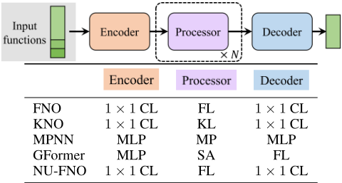
The 12 ON models are classified into three types according to their different encoder-processor-decoder (EPD) architectures: (1) EPD with a single encoder and a single decoder, (2) EPD with multi-encoder and a single decoder; and (3) EPD with U-shaped architectures(multi-encoder and multidecoder).
The first type of models is illustrated in Figure 1. These models can be uniformly described as first concatenating all input data (e.g., initial/boundary conditions and parameters) into a single representation, which is then encoded into a latent space using a single encoder. After processing, the latent features are finally decoded back into the observable space through a single decoder. Various architectures can be employed to parameterize the encoder and decoder, including MLP, 1×1 convolution, and Fourier layer, as utilized in this type. For the core processor, both FNO and KNO adopt a divide-and-conquer strategy to separately handle high-frequency and low-frequency information, with FNO using Fourier layers and KNO employing Koopman layers for high-frequency processing. MPNN employs a graph neural network (GNN) based on message passing, while GFormer introduces a processor with a non-Softmax selfattention mechanism (Fourier/Galerkin-type attention). NU- FNO shares the same EDP as FNO, but it includes conversions between nonuniform and uniform grids both before and after the EDP.
| UPS | MLP | FL | LLM | MLP |
|---|---|---|---|---|
| DeepONet | MLP | MLP | DP | - |
| OFormer | MLP | MLP + SA | CA+MLP | MLP |
| GNOT | MLP | MLP | CA+ SA | MLP |
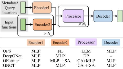
The second type of models is illustrated in Figure 2. In addition to input function encoders, this type of models includes a text metadata encoder in UPS and a query positions encoder in the other three models. Specifically, the foundation model UPS utilizes the embedder of an LLM to process metadata, including problem descriptions and physical parameters, while variable data are encoded using Fourier layers. The concatenated features from both parts are fed into the LLM-based processor. Moreover, the remaining three models use MLP as encoders and decoders, with OFormer incorporating self-attention in the encoder. For the number of input function encoders, N1 = 1 in DeepONet and OFormer, while N1 > 1 in GNOT, allowing separate encoding of multiple types of input functions. After encoding, DeepONet transfers the information of the input functions to the query points through a dot product operation, while OFormer and GNOT use cross-attention mechanisms to achieve this. Notably, when solving time-dependent PDE systems, OFormer introduces an additional processor (MLP) to predict the residual of the solution between each time step in the latent space, which differs from the way the other 11 models propagate dynamics in the observable space.
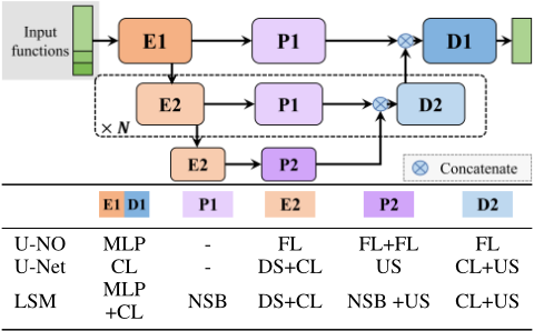
The third type of models is illustrated in Figure 3. These models are based on a U-shaped architecture, consisting of a contracting path (left side) and an expansive path (right side), with skip connections from the encoder to the decoder. Specifically, the first encoder and final decoder of these three models offer three options: MLP, 1×1 convolution, and two 3×3 convolutions. In other parts of the model architecture, UNO primarily uses nonlinear integral operators (Fourier layers), with the left encoder reducing the domain size and increasing the co-domain dimension, while the right decoder performs the opposite operation. U-Net is mainly based on two 3×3 convolutions, with the left encoder performing downsampling and the right decoder handling upsampling. With the same architecture as the U-Net, LSM incorporates a neural spectral block design in the processor. The block involves the following steps: first, high-dimensional data is projected into a latent space using a hierarchical projection network based on cross-attention. The PDE is then solved in this latent space. Afterward, the data are projected back to the original coordinate space. Patchify and de-patchify operations are applied at the beginning and end of the process, respectively.
3.4 EvaluationMetrics
The CFDONEval metrics include 3 accuracy metrics, 2 time metrics, and 3 visualization metrics. Below is a brief explanation of how to calculate these metrics. The three accuracy metrics are calculated with the formulae
where (yi)ni=1 represents the ground truth, (ˆ yi)ni=1 represents the predictions, and n is the number of test cases. The time metrics include training time ttrain and inference time tinfer. The training time ttrain is calculated with the formula ttrain = Nepoch × tepoch, where tepoch is the time spent to train the model for one epoch, Nepoch represents the number of epochs required for training. The inference time tinfer is the average time to predict one time step's solution for all samples in the test dataset, calculated by tinfer = tframe/k, where tframe is the total inference time for all samples in the test dataset, and k is the number of samples. Finally, three visualization metrics include the kinetic energy spectrum metric KES, the flow streamline metric FSV and contours metric FCV. The KES describes the distribution of kinetic energy across different wave numbers (scales) and is widely used in multiscale modeling, its evaluation algorithm and the computation script is from [Navah et al., 2020] and [Navah, 2024], respectively. The FSV visually displays the fluid flow paths and directions, allowing us to visually assess whether the evaluated ON models accurately predict fluid flow phenomena, such as the symmetry, size, and number of vortices. The FCV refers to contour lines or surfaces that represent constant values of a flow field variable, such as velocity or pressure, within a fluid flow. These contours help visualize the distribution and variation of the variable across the flow domain.
4 Performance of Models
To evaluate the 12 ON models (see Section 3.3), we conducted extensive experiments, training them on 22 datasets (see Section 3.2) and 9 novel datasets derived from combinations of the original 22. The performance was assessed using 8 metrics (see Section 3.4). All experiments were conducted on two Intel Xeon Platinum 8375C CPUs @ 2.90GHz, one NVIDIA GeForce RTX 4090 GPU, with PyTorch 2.1.2 and CUDA 11.8. Due to space constraints, we present only a selection of representative results showing the performance of ON models in addressing Challenge C1 to C5 with a few metrics here. Other evaluation results are presented in Appendix E. Notably, the training loss for all models is based on the error between the ground truth and the predicted values across three consecutive time steps. During testing, the trained models are provided with data from the initial time step, and the predicted results for each subsequent time step are evaluated. The three accuracy metrics are computed by averaging the cumulative error across all time steps.
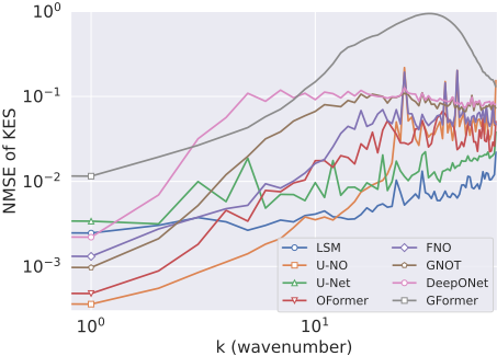
On Multiscale phenomena (C1). Figure 4 shows the normalized mean squared error (NMSE) of the KES between the predictions of the 8 ON models and the ground truth, trained on the DARP2 dataset. The results for the remaining 4 models are not included, as they are unable to solve time-independent problems. The NMSE for each wavenumber is averaged over all test sequences. The results show that all models achieve higher simulation accuracy at low wavenumbers (large scales) compared to high wavenumbers (small scales). In the lowwavenumber range (wavenumber < 10), U-NO performs the best, followed by LSM, OFormer, FNO, U-Net, GNOT, DeepONet and GFormer. In the high wavenumber range, LSM performs the best, followed by UNet, the remaining models show relatively poorer performance, with errors greater than 0.01. Overall, LSM demonstrates stable performance, maintaining errors below 0.01 across most wavenumbers, except for a few specific cases.
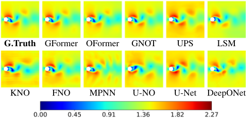
On Convection dominance (C2). Figure 5 illustrates the contours of velocity field predictions at t = 2.2 for a Reynolds number Re = 100, 000 in the CCFRe dataset, where convection effects dominate the flow. We observe that the models GFormer and OFormer excel in predicting both the velocity magnitude and the flow field phenomena, including the K´arm´an vortex street. The models GNOT, UPS, and LSM also demonstrate good performance in predicting flow field phenomena, though some errors are observed in predicting the velocity magnitude. In comparison, KNO, FNO, and MPNN show slightly reduced performance, with lower accuracy in predicting the velocity magnitude. Furthermore, the U-NO, U-Net, and DeepONet models exhibit errors not only in predicting the velocity magnitude but also in capturing the direction of vortex rotation.
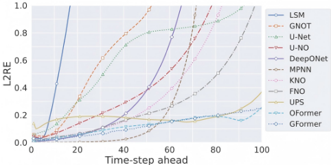
On Long-term predictions (C3). Figure 6 presents the L2RE error curve for the TGVRe dataset at different time steps. We evaluate the model's predictions over up to 100 time steps, which significantly exceeds the maximum 3-frame prediction horizon during training. The L2RE for each time step is calculated by averaging over all cases in the test set with more than 100 time steps. All models, except UPS, perform well in the first five time steps, with errors below 0.1. The results show that, the models GFormer and OFormer perform the best, with their L2RE error consistently staying below 0.3 throughout the entire prediction range. The error also increases very gradually and almost linearly. The UPS also performs well, maintaining an error below 0.2 for the first 80 time steps, demonstrating high stability. The FNO, KNO, and DeepONet perform moderately, with errors reaching 0.1 after 30 time steps, after which the error growth rate increases. The MPNN maintains very low errors up to 40 time steps, but the error increases sharply after 50 time steps. The error curve for U-NO gradually rises, but the error remains below 0.4 within 50 frames. U-Net, GNOT, and LSM show relatively poorer performance, with errors reaching 0.8 at approximately 50, 40, and 15 time steps, respectively. Among these, the LSM exhibits the steepest error trend, with the error increasing sharply to 1 within the first 20 time steps.
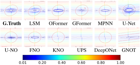
On Multiphase (C4). Figure 7 compares the predicted streamlines of the ON models with the ground truth at t = 0.35 for the sample Mo = 0.005 in dataset TPFMo. The phase interface is outlined with contours, highlighted in red. We observe that LSM successfully simulates the deformation of the interface along the flow direction and accurately captures the formation of vortices inside the interface. Additionally, the OFormer and GFormer simulate slight deformations of the interface, followed by MPNN, U-Net, U-NO, FNO, KNO, and UPS. The UPS model is unable to handle variables not included in the remaining datasets, which is why it does not predict the two-phase interface. DeepONet struggles to predict the vortices within the interface, while GNOT cannot simulate the two-phase interface.
On unstructured meshes over complex geometries (C5). Table 2 lists the L2RE predictions made by the 6 ON models, trained on three datasets with unstructured meshes. Overall, the results show that NU-FNO performs exceptionally well, achieving the lowest L2RE errors in both velocity and pressure predictions across the three datasets multiple times. Similarly, GNOT also performs excellently, consistently ranking in the top 3 for prediction accuracy, with the lowest prediction errors for the x-direction velocity u on both the CCF∗Re and PHF∗Re datasets. Models that perform slightly weaker include MPNN, OFormer, and DeepONet. LSM, however, does not performwell in this challenge.
| Dateset | MPNN | NU-FNO | DeepONet | OFormer | GNOT | LSM | |
|---|---|---|---|---|---|---|---|
| CCF∗Bc | u v p | 1.82E-01 9.70E-01 5.74E-01 | 8.28E-02 9.82E-02 2.69E-02 | 1.92E-01 8.41E-01 2.33E+00 | 1.57E-01 8.13E-01 4.14E-01 | 1.49E-01 7.56E-01 3.86E-01 | 1.69E-01 7.39E-01 1.07E+00 |
| CCF∗Re | u v p | 9.14E-02 2.08E-01 2.69E-01 | 1.08E-01 8.88E-02 3.83E-02 | 1.27E-01 4.98E-01 3.96E-01 | 1.09E-01 5.75E-01 2.29E-01 | 7.07E-02 3.34E-01 1.69E-01 | 2.63E-01 8.07E-01 4.57E-01 |
| PHF∗Re | u v w p | 1.72E-01 1.23E+00 7.75E-01 6.08E-01 | 3.54E-01 4.14E-02 5.73E-02 1.26E-01 | 7.63E-01 1.04E+00 9.95E-01 8.41E-01 | 1.96E-01 1.36E+00 8.32E-01 4.68E-01 | 1.61E-01 1.20E+00 7.26E-01 4.58E-01 | - - - - |
5 Conclusions
The results of evaluation experiments conducted in CFDONEval demonstrate the crucial impact of network architecture on the predictive performance of neural network models for CFD problems, while also showing the important role of data quality and preprocessing before model training.
First, network architecture plays a critical role in determining model performance. Each model of the first type has a single encoder and decoder, with simple structures such as MLP or a 1×1 convolutional layer. Its predictive performance is primarily influenced by the choice of processor. FNO and KNO excel in short-term predictions, likely due to their ability to separately handle high- and low-frequency information, compensating for the common ON's limitation of better learning low-frequency features than high-frequency ones. MPNN performs exceptionally well in making shortto medium-term forecasts, probably because its processor, through message passing, can more readily extract local features. GFormer performs exceptionally well in tackling Challenges C2 and C3, probably because its processor self attention facilitates the extraction of global features more effectively. A model of the second type differs from one in the first type mainly by incorporating an additional encoder for special purposes. The additional encoders of the models DeepONet, OFormer, GNOT are designed to handle query locations, enabling queries at arbitrary locations independent of the input grid points, which enhances the flexibility of the models and improves their prediction performance. For instances, DeepONet performs well in large-scale flow predictions and short-term forecasting, OFormer excels in addressing Challenges C2 and C3, GNOT excels in addressing Challenge C5 and demonstrates above-average performance in solving Challenge C2. The additional encoder of the UPS is designed to handle text metadata describing physical parameters or governing equations. UPS performs well on both Challenges C2 and C3, demonstrating stable performance across tasks. Models of the third type all have a U-shaped structure, extracting features at different scales, so they have advantages in handling Challenge C1. Their performance varied on other Challenges, such as LSM outperforms both U-NO and U-Net in Challenge C2.
On the other hand, models based on transformer architectures perform exceptionally well in Challenges C2, C3 and C4, and above average in Challenges C1. Their superior performance may be attributed to their ability to effectively capture long-range dependencies and complex spatial correlations inherent in convection-dominated flows. As a fundamental GNN model, MPNN has shown strong performance in short- to medium-term predictions. Exploring more advanced GNN architectures for CFD represents a promising and worthwhile research direction. As a foundation model, UPS performs stably across all challenges, particularly excelling in Challenges C2 and C3. Future work should pay more attention to design more advantageous foundation models which can handle more diverse input data and more types of fluid problems and have superior predictive performance. In processing unstructured data, NU-FNO delivers the best performance in multiple tasks related to Challenge C5, due to its specialized interpolation techniques. On the other hand, models like GNOT can directly process unstructured data and perform well. How to process unstructured data in the future is still a question worth exploring.
Secondly, data is another critical factor affecting the performance of ON models. The quality and quantity of training data significantly impact model performance, but generating a large volume of high-quality data requires substantial computational resources. Finding the balance between computational cost and improving the quality of large-scale data is a crucial issue. Alternatively, combining a small amount of high-fidelity data with a large amount of low-fidelity data for training may be an effective strategy to improve models' performance. Furthermore, employing appropriate data preprocessing methods can also significantly enhance the models' predictive performance.
Acknowledgments
This work was supported by the National Science and Technology Major Project (2022ZD0117805), by the National Natural Science Foundation of China under grants 92370113 and 12201369, and by the Guangdong Provincial Key Laboratory of Mathematical Foundations for Artificial Intelligence (2023B1212010001).
@inproceedings{ijcai2025p640,
  title     = {CFDONEval: A Comprehensive Evaluation of Operator-Learning Neural Network Models for Computational Fluid Dynamics},
  author    = {Liu, Menghan and Cen, Jianhuan and Zhou, Ziyang and Fan, Haolong and Li, Hongji and Wei, Ping and Peng, Guohang and He, Changye and Qin, Yuzhe and Lu, Yutong and Zou, Qingsong},
  booktitle = {Proceedings of the Thirty-Fourth International Joint Conference on
               Artificial Intelligence, {IJCAI-25}},
  publisher = {International Joint Conferences on Artificial Intelligence Organization},
  editor    = {James Kwok},
  pages     = {5752--5760},
  year      = {2025},
  month     = {8},
  note      = {Main Track},
  doi       = {10.24963/ijcai.2025/640},
  url       = {https://doi.org/10.24963/ijcai.2025/640},
}
TY - CPAPER TI - CFDONEval: A Comprehensive Evaluation of Operator-Learning Neural Network Models for Computational Fluid Dynamics AU - Liu, Menghan AU - Cen, Jianhuan AU - Zhou, Ziyang AU - Fan, Haolong AU - Li, Hongji AU - Wei, Ping AU - Peng, Guohang AU - He, Changye AU - Qin, Yuzhe AU - Lu, Yutong AU - Zou, Qingsong T2 - Proceedings of the Thirty-Fourth International Joint Conference on Artificial Intelligence, IJCAI-25 PB - International Joint Conferences on Artificial Intelligence Organization PY - 2025 SP - 5752 EP - 5760 DO - 10.24963/ijcai.2025/640 UR - https://doi.org/10.24963/ijcai.2025/640 ER -Copied
Machine-readable versions of this paper, for tools and AI agents:





