
Capturing Individuality and Commonality Between Anchor Graphs for Multi-View Clustering
Proceedings of the Thirty-Fourth International Joint Conference on Artificial Intelligence. Main Track. Pages 5860-5868.
https://doi.org/10.24963/ijcai.2025/652
Keywords
- Machine Learning: ML: Unsupervised learning
- Machine Learning: ML: Multi-view learning
- Machine Learning: ML: Clustering
Abstract
The use of anchors often leads to better efficiency and scalability, making them highly favored. However, there is a challenge in anchor-based multi-view subspace learning. A unified anchor graph overly emphasize the commonality between views, failing to adequately capture the view-specific individuality. This has led some models to independently explore the individuality of each view before aligning and integrating them, often achieving better performance but making the process more cumbersome. Therefore, this paper proposes a new model, simultaneously capturing the individuality and commonality between anchor graphs for multi-view clustering. The model has three notable advantages: First, it allows view-specific anchor graphs to align in real-time with a common anchor graph as a reference, eliminating the need for post-alignment. Second, it enforces a cluster-wise structure among anchors and balances sample distribution among them, providing strong discriminative power. Lastly, it maintains linear complexity with respect to the numbers of samples and anchors, avoiding the significant time costs associated with their increase. Comprehensive experiments demonstrate the effectiveness and efficiency of our method compared to various state-of-the-art algorithms.
- [Baltrušaitis et al., 2018] Tadas Baltrušaitis, Chaitanya Ahuja, and Louis-Philippe Morency. Multimodal machine learning: A survey and taxonomy. IEEE Transac- tions on Pattern Analysis and Machine Intelligence, 41(2):423-443, 2018.
- [Chen et al., 2022] Man-Sheng Chen, Chang-Dong Wang, Dong Huang, Jian-Huang Lai, and Philip S Yu. Efficient orthogonal multi-view subspace clustering. In Proceed- ings of the ACM SIGKDD Conference on Knowledge Dis- covery and Data Mining, pages 127-135, 2022.
- [Fang et al., 2023] Uno Fang, Man Li, Jianxin Li, Longxi- ang Gao, Tao Jia, and Yanchun Zhang. A comprehensive survey on multi-view clustering. IEEE Transactions on Knowledge and Data Engineering, 35(12):12350-12368, 2023.
- [Gao et al., 2020] Quanxue Gao, Wei Xia, Zhizhen Wan, Deyan Xie, and Pu Zhang. Tensor-svd based graph learn- ing for multi-view subspace clustering. In Proceedings of the AAAI Conference on Artificial Intelligence, volume 34(04), pages 3930-3937, 2020.
- [Huang et al., 2022] Shudong Huang, Hongjie Wu, Yazhou Ren, Ivor Tsang, Zenglin Xu, Wentao Feng, and Jiancheng Lv. Multi-view subspace clustering on topological mani- fold. Advances in Neural Information Processing Systems, 35:25883-25894, 2022.
- [Kang et al., 2020] Zhao Kang, Wangtao Zhou, Zhitong Zhao, Junming Shao, Meng Han, and Zenglin Xu. Large- scale multi-view subspace clustering in linear time. In Pro- ceedings of the AAAI Conference on Artificial Intelligence, volume 34(04), pages 4412-4419, 2020.
- [Li et al., 2018] Yingming Li, Ming Yang, and Zhongfei Zhang. A survey of multi-view representation learning. IEEE Transactions on Knowledge and Data Engineering, 31(10):1863-1883, 2018.
- [Li et al., 2022a] Xingfeng Li, Yinghui Sun, Quansen Sun, and Zhenwen Ren. Consensus cluster center guided la- tent multi-kernel clustering. IEEE Transactions on Cir- cuits and Systems for Video Technology, 33(6):2864-2876, 2022.
- [Li et al., 2022b] Xuelong Li, Han Zhang, Rong Wang, and Feiping Nie. Multiview clustering: A scalable and parameter-free bipartite graph fusion method. IEEE Trans- actions on Pattern Analysis and Machine Intelligence, 44(1):330-344, 2022.
- [Liu et al., 2021] Jiyuan Liu, Xinwang Liu, Yuexiang Yang, Li Liu, Siqi Wang, Weixuan Liang, and Jiangyong Shi. One-pass multi-view clustering for large-scale data. In Proceedings of the IEEE/CVF International Conference on Computer Vision, pages 12344-12353, 2021.
- [Liu et al., 2024] Suyuan Liu, Ke Liang, Zhibin Dong, Siwei Wang, Xihong Yang, Sihang Zhou, En Zhu, and Xinwang Liu. Learn from view correlation: An anchor enhance- ment strategy for multi-view clustering. In Proceedings of the IEEE/CVF Conference on Computer Vision and Pat- tern Recognition, pages 26151-26161, 2024.
- [Liu, 2022] Xinwang Liu. SimpleMKKM: Simple multiple kernel k-means. IEEE Transactions on Pattern Analysis and Machine Intelligence, 45(4):5174-5186, 2022.
- [Wan et al., 2023] Xinhang Wan, Xinwang Liu, Jiyuan Liu, Siwei Wang, Yi Wen, Weixuan Liang, En Zhu, Zhe Liu, and Lu Zhou. Auto-weighted multi-view clustering for large-scale data. In Proceedings of the AAAI Conference on Artificial Intelligence, volume 37(8), pages 10078- 10086, 2023.
- [Wang et al., 2022a] Siwei Wang, Xinwang Liu, Suyuan Liu, Jiaqi Jin, Wenxuan Tu, Xinzhong Zhu, and En Zhu. Align then fusion: Generalized large-scale multi-view clustering with anchor matching correspon- dences. Advances in Neural Information Processing Sys- tems, 35:5882-5895, 2022.
- [Wang et al., 2022b] Siwei Wang, Xinwang Liu, Xinzhong Zhu, Pei Zhang, Yi Zhang, Feng Gao, and En Zhu. Fast parameter-free multi-view subspace clustering with con- sensus anchor guidance. IEEE Transactions on Image Pro- cessing, 31:556-568, 2022.
- [Wen et al., 2023] Yi Wen, Suyuan Liu, Xinhang Wan, Si- wei Wang, Ke Liang, Xinwang Liu, Xihong Yang, and Pei Zhang. Efficient multi-view graph clustering with lo- cal and global structure preservation. In Proceedings of the ACM International Conference on Multimedia, pages 3021-3030, 2023.
- [Xia et al., 2022] Wei Xia, Quanxue Gao, Qianqian Wang, Xinbo Gao, Chris Ding, and Dacheng Tao. Tensorized bipartite graph learning for multi-view clustering. IEEE Transactions on Pattern Analysis and Machine Intelli- gence, 45(4):5187-5202, 2022.
- [Xu et al., 2022] Jie Xu, Huayi Tang, Yazhou Ren, Liang Peng, Xiaofeng Zhu, and Lifang He. Multi-level feature learning for contrastive multi-view clustering. In Proceed- ings of the IEEE/CVF Conference on Computer Vision and Pattern Recognition, pages 16051-16060, 2022.
- [Yan et al., 2023] Weiqing Yan, Yuanyang Zhang, Chenlei Lv, Chang Tang, Guanghui Yue, Liang Liao, and Weisi Lin. GCFAgg: Global and cross-view feature aggregation for multi-view clustering. In Proceedings of the IEEE/CVF Conference on Computer Vision and Pattern Recognition, pages 19863-19872, 2023.
- [Zhang et al., 2023] Pei Zhang, Siwei Wang, Liang Li, Changwang Zhang, Xinwang Liu, En Zhu, Zhe Liu, Lu Zhou, and Lei Luo. Let the data choose: Flexible and diverse anchor graph fusion for scalable multi-view clus- tering. In Proceedings of the AAAI Conference on Artificial Intelligence, volume 37(9), pages 11262-11269, 2023.
- [Zhang et al., 2024] Chao Zhang, Xiuyi Jia, Zechao Li, Chunlin Chen, and Huaxiong Li. Learning cluster-wise anchors for multi-view clustering. In Proceedings of the AAAI Conference on Artificial Intelligence, volume 38(15), pages 16696-16704, 2024.
References were extracted automatically from the PDF and may contain errors.
Full text extracted automatically from the PDF; figures, tables and equations may differ. The PDF is the version of record.
1 Introduction
Clustering has long been a crucial aspect of data analysis, which groups data according to specific patterns without label information. The emergence of multi-source data [Baltruˇsaitis et al., 2018] has raised higher demands for clustering tasks, giving rise to multi-view extension [Li et al., 2018; Fang et al., 2023]. In this setting, data often comes with multiple perspectives or representations. The consistent and complementary information among these views is explored to address the limitations of single-view information and enhance performance.
∗Corresponding author
Multi-view clustering can be roughly categorized into subspace-based [Gao et al., 2020; Huang et al., 2022], kernelbased [Li et al., 2022a; Liu, 2022], matrix factorization-based [Wan et al., 2023], and deep learning-based [Xu et al., 2022; Yan et al., 2023] methods. Subspace clustering is widely recognized as an effective data analysis technique, as it can directly learn affinities between samples, revealing the internal structure of the data. Unfortunately, it often struggles with the high computational costs associated with large-scale datasets.
On the other hand, the use of anchors has brought about better efficiency and scalability, making them highly popular. Naturally, this technology has been integrated into subspace learning models. In anchor-based subspace learning, a point-to-anchor graph is learned instead of a point-to-point graph. Since the number of anchors is usually much smaller than that of samples, it is more friendly to both runtime and memory. Anchors can be pre-selected, resorting to heuristic strategies such as k-means and feature scoring. However, these pre-selection strategies face the risk of being insufficient to represent the entire dataset, which leads to dynamic anchor learning strategies.
However, a challenge arises in anchor-based multi-view subspace learning. A unified anchor graph tends to overemphasize the commonality between views, failing to adequately capture the individuality of each view. This has led some models to independently explore each view's individuality before aligning and integrating them, often achieving better performance but making the process more cumbersome. Moreover, although existing models maintain linear complexity with respect to the number of samples, they often exhibit quadratic or even cubic complexity with respect to the number of anchors. The growth of anchors inevitably results in substantial time costs.
To address these issues, this paper proposes a new model, Capturing Individuality and Commonality between Anchor Graphs (CICAG) for multi-view clustering. The four contributions are summarized as follows:
- It captures both the individuality and commonality between anchor graphs, addressing the limitations of previous approaches that focus solely on either aspect.
- It enables view-specific anchor graphs to align in realtime with a common anchor graph as a reference, eliminating the need for post-alignment.
- It enforces a cluster-wise structure among anchors and balances samples distribution among them, providing strong discriminative power.
- It achieves linear computational complexity concerning both the number of samples and anchors, making it efficient and scalable even with a large number of anchors.
2 RelatedWork
Anchor-based multi-view learning models can be categorized into two main types: static anchor pre-selection and dynamic anchor learning. The former determine anchors in advance using heuristic methods, with no changes during subsequent anchor graph construction. The latter requires joint optimization of anchors and anchor graphs with dynamic updates. Dynamic anchor learning includes unified anchor graph strategies, which share a common anchor graph across all views, and view-specific anchor graph strategies, which learn a separate anchor graph for each view.
LMVSC [Kang et al., 2020] employs k-means to pre-select anchors for each view and constructs non-unified anchor graphs, which are then concatenated across views. SFMC [Li et al., 2022b] and TBGL [Xia et al., 2022] pre-select aligned anchors by concatenating all features and using a feature scoring strategy, subsequently merging multiple anchor graphs. Unlike SFMC, TBGL utilizes tensors to further explore complementary information across views.
FPMVS-CAG [Wang et al., 2022b], OMSC [Chen et al., 2022], EMVGC-LG [Wen et al., 2023], and CAMVC [Zhang et al., 2024] are representative models, dynamically exploring a unified anchor graph. FPMVS-CAG projects all views into a latent shared space to learn a single anchor graph. OMSC builds on FPMVS-CAG by jointly learning the mapping from the anchor graph to the cluster indicator matrix. EMVGC-LG embeds both local and global structural information into the anchor graph. CAMVC uses pseudo-labels to enforce cluster structure distribution among anchors.
FMVACC [Wang et al., 2022a], FDAGF [Zhang et al., 2023], and AEVC [Liu et al., 2024] are based on anchorbased subspace learning models, capturing separate anchor graphs for different views. FMVACC and AEVC both employ post-alignment strategies, whereas FDAGF directly concatenates anchor graphs from each view. Unlike FMVACC, which averages after alignment, AEVC embeds the learned anchors and anchor graphs into a new model for secondary learning, serving as regularization.
3 Methodology
3.1 Formulation
Typically, the framework for single-view subspace learning takes the following form.
where X ∈ Rd×n represents the complete single-view dataset, A ∈ Rd×m is a representative subset of samples, Z ∈ Rm×n is the weight matrix used to linearly combine A to reconstruct X, n, m and d are the number of samples, anchors and features, respectively. More concisely, A and Z can be referred to as the anchors and anchor graph, respectively. The anchor graph describes an affinity between X and A. As a multi-view extension strategy, a unified anchor graph is often required, resulting in the following form.
where Z is the anchor graph shared across views, while X(i) and A(i) denote the samples and anchors of the i-th view, respectively. Regrettably, this form overly emphasizes the commonality between views and fails to adequately capture the individuality of each view, thus giving rise to another form.
where Z(i) is the anchor graph unique to the i-th view. This case independently explores the individuality of each view before aligning and integrating them, often achieving better performance, but also making the process more cumbersome. Therefore, we propose a compromise solution.
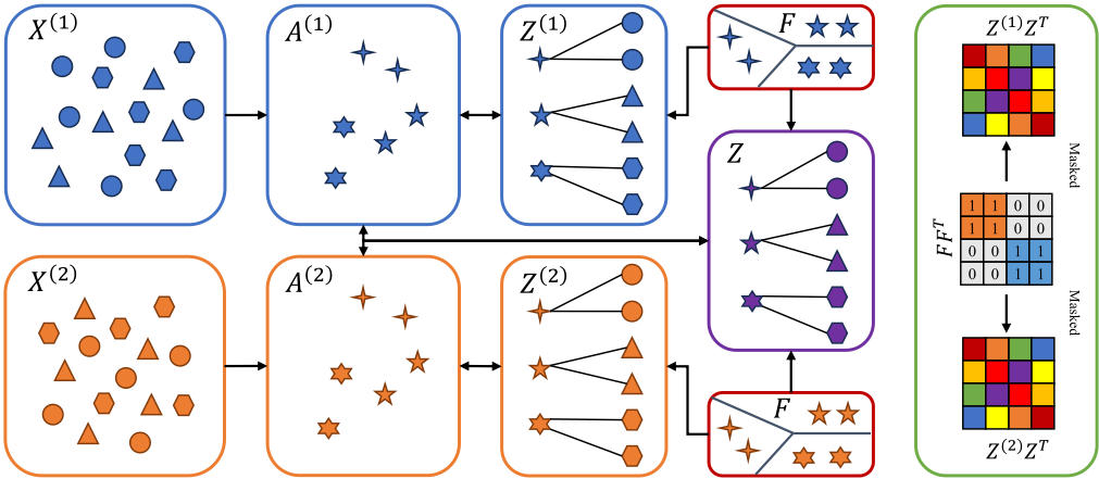
In this approach, we not only extract a common Z for all views but also exploit a specific Z(i) for each view. The anchor set A(i) are shared between Z(i) and Z, ensuring that Z(i) and Z are well-aligned. Indirectly, through the assistance of Z, this alignment relationship is shared among Z(i) .
Meanwhile, the anchors are desired to be evenly distributed across the clusters and further aligned. Thus, the following strategy is adopted.
where F ∈ Rm×c is a predefined anchor-to-cluster assignment matrix, with each cluster containing at least ⌊m/c⌋ and at most ⌈m/c⌉ anchors. For instance, if there are 4 anchors and 2 clusters, then F is set as
Next, we further consider the constraints regarding several variables. If A(i) can effectively represent X(i) , the following equality holds.
This equation implies a series of simpler non-trivial solutions, which necessitate the orthogonality of A(i) .
It is suggested to more freely retain the individuality of Z(i) , only with each row summing to 1.
Meanwhile, Z must ensure a more balanced distribution of samples among anchors, subject to the following constraint.
Considering Problems 4-5 and Constraints 8-10, the final objective function is formulated as follows:
Figure 1 illustrates our proposed CICAG framework. It dynamically captures an individual anchor graph Z(i) for each view's data X(i) while simultaneously exploring a common anchor graph Z for all views. Z(i) and Z share a dynamic anchor set A(i) , thus enabling indirect real-time alignment between individual anchor graphs. Meanwhile, a predefined anchor-to-cluster assignment matrix F enforces the clusterwise structure among anchors and enhances alignment. Additionally, the common anchor graph requires a more balanced distribution of samples across the anchors.
3.2 Optimization
To solve our model, the following alternating optimization strategy is employed.
Update A(i)
If the components unrelated to A(i) are removed andW (i) is precomputed as
the resulting A(i) -subproblem is given.
Furthermore, the closed-form solution for Equation (13) can be revealed by Theorem 1 [Liu et al., 2021].
Theorem 1. Suppose that W (i) = U (i) c Σ(i) c V (i)T c , where U (i) c ∈ Rdi×c , Σ(i) c ∈ Rc×c and V (i) c ∈ Rm×c . Problem 13 has a closed-form solution A(i) = U (i) c V (i)T c .
Update Z(i)
If the components unrelated to Z(i) are removed, and ˜E(v) and E(v) are precomputed as
the resulting Z(i) -subproblem is given.
Furthermore, the optimal solution for Equation (16) can be revealed by Theorem 2.
Theorem 2. By introducing the Lagrange multiplier µ(i) and predefining S(i) and Φ(S(i) ) as
the dual problem of Problem 16 is derived as
whose exact gradient with respect to µ(i) is given by
Once the optimal µ(i) is found, the desired Z(i) can be recovered by
Proof. Similar to the proof of Theorem 3 but simpler.
Update Z
If the components unrelated to Z are removed, and ˜M (i) and M are precomputed as
the resulting Z-subproblem is given.
Furthermore, the optimal solution for Equation (24) can be revealed by Theorem 3.
Theorem 3. By introducing the Lagrange multipliers µ and ν, and predefining S and Φ(S) as
the dual problem of Problem 24 is
whose exact gradients with respect to µ and ν are given by
Once the optimal µ and ν are found, the desired Z can be recovered by
Proof. The following min-max problem is given
(31)
which is easily transformed into the max-min form.
Further, there are the following max-max problems
Obviously, Equation (33) is equivalent to Equation (27). In addition, split Φ(S) by column as
it is easy to konw the derivatives as
Further, its gradients w.r.t. µ and ν can be computed.
Final Fusion
Once our model converges, the desired anchor graph is obtained by Equation (36). For convenience, our methodological procedure is summarized in Algorithm 1.
Algorithm 1 CICAG Solver
Input: Dataset {X(i) }vi=1 , anchor number m, cluster number c, and parameters α, β and γ.
Output: Learned anchor graph Z∗ .
- 1: Initialize Z(i) ,Z and F.
- 2: while non-convergence do
- 3: Update A(i) by Theorem 1.
- 4: Update Z(i) by Theorem 2.
- 5: Update Z by Theorem 3.
- 6: end while
- 7: Obtain Z∗ by Equation (36).
3.3 Complexity
TimeComplexity. In theA(i) -subproblem, computingW (i) and obtaining its singular value decomposition necessitates O(nmd+mdc), while updating A(i) only costs O(mdc). In the Z(i) -subproblem, computing ˜E(i) and E(i) together involves O(nmd + nmc), obtaining the gradient with respect to µ(i) entails O(nm), and updating µ(i) and Z(i) involves O(n) and O(nm) respectively. In the Z-subproblem, computing M demands O(nmd+nmcv), obtaining the gradients with respect to µ and ν both necessitate O(nm), and updating µ, ν, and Z entails O(n), O(m), and O(nm) respectively. Thus, in one iteration, our model requires a computational complexity of only O(nmd + nmcv + mdc), which implies that our algorithm is not only linear in the number of samples n, but also linear in the number of anchors m, data dimension d, and the number of clusters c. Table 1 lists some notable algorithms whose complexities often reach quadratic or even cubic with respect to m, which actually limits their scalability. Additionally, the complexity of some algorithms with respect to c is not linear, making them less suitable for data with a large number of clusters.
| Method | Computational Complexity |
|---|---|
| LMVSC SFMC TBGL FPMVS OMSC FMVACC FDAGF EMVGCLG AEVC CAMVC CICAG | O(nmc + nmd + mdc) O(nm2 + nmd + nmc + m3 ) O(nm2 + nm log n + nmc + nmd) O(nm3 + nmd) O(nm3 +m2 c +mc3 +nmc +dc3 ) O(nm2 + nmd + m2d + m3 ) O(nm2 + nmd + m2d) O(nm3 + nmd) O(nm3 + nmd) O(nm2 c2 +nmdc +m3 c3 +m2 c2d) O(nmd + nmc + mdc) |
Space Complexity. The original data {X(i) } consumes O(nd) space. The auxiliary variables generated from updating A(i) necessitate O(md), and A(i) also takes up O(md). The auxiliary variables generated from updating Z(i) require O(nmv), and Z(i) also takes up O(nmv). The auxiliary variables generated from updating Z demand O(nm) space, and Z itself also uses O(nm). Therefore, our algorithm needs only O(nd + md + nmv) space complexity, which is typical for anchor-based methods.
3.4 Convergence
Although the overall objective function, involving multiple variables, is non-convex, fortunately, each subproblem concerning a single variable is convex. For the A(i) -subproblem, a closed-form solution exists. For the Z(i) -subproblem and the Z-subproblem, their equivalent dual problems can be constructed. Since the exact gradients of the dual problems can be obtained, any gradient-based method can be used to find their optimal solutions. Let the objective function value at the t-th iteration be J({A(i) t }, {Z(i) t },Zt), then the following inequality holds.
Obviously, since the function value monotonically decreases with each iteration and has a lower bound, this algorithm can ensure convergence to a local minimum.
4 Experiment
4.1 Experimental Protocols
Datasets. Our experiments employ 9 public datasets for comparison, including 3Sources, WebKB, NUS-WIDE, NottingHill, Cifar10, Cifar100, YouTubeFace10, YouTubeFace20 and YouTubeFace50. Specifically, the last five are large-scale datasets. Their statistics are described in Table 2.
| Dataset | #Views | #Instances | #Classes | #Features |
|---|---|---|---|---|
| 3Sources | 3 | 169 | 3 | 3560, 3631, 3068 |
| WebKB | 2 | 1051 | 2 | 2949, 334 |
| NUS-WIDE | 5 | 3000 | 25 | 64, 225, 144, 73, 128 |
| Notting-Hill | 3 | 4660 | 5 | 6750, 3304, 2000 |
| Cifar10 | 3 | 50000 | 10 | 512, 2048, 1024 |
| Cifar100 | 3 | 50000 | 100 | 512, 2048, 1024 |
| YouTubeFace10 | 4 | 38654 | 10 | 944, 576, 512, 640 |
| YouTubeFace20 | 4 | 63896 | 20 | 944, 576, 512, 640 |
| YouTubeFace50 | 4 | 126054 | 50 | 944, 576, 512, 640 |
Baselines. Our CICAG is compared with the following 9 algorithms: SFMC [Li et al., 2022b], TBGL [Xia et al., 2022], FPMVS [Wang et al., 2022b], OMSC [Chen et al., 2022], FMVACC [Wang et al., 2022a], FDAGF [Zhang et al., 2023], EMVGC [Wen et al., 2023], CAMVC [Zhang et al., 2024] and AEVC [Liu et al., 2024]. These classic or state-of-the-art algorithms are highly correlated with ours and have a nearlinear computational complexity.
Settings. For our model, α is set to 0.1, while the remaining hyperparameters are tuned by a grid search, whose ranges are m ∈ {1c, 3c, 5c}, β ∈ {0.001, 0.01, · · · , 100, 1000}, and γ ∈ {0.001, 0.01, · · · , 100, 1000}. The hyperparameters of all compared algorithms are set by gird search according to the recommendations of their original papers. Considering the initialization sensitivity and randomness during running, we performed all algorithms 10 times.
Metrics. In our experiments, the performance is evaluated by Accuracy (ACC), Normalized Mutual Information (NMI) and Adjusted Rand Index (ARI). Their means and standard deviations are reported in experiments. Besides, their average runtime is also recorded.
4.2 Experimental Results
Performance. Table 3 shows, CICAG achieves the highest ACC across all used datasets, with its NMI and ARI being either the highest or second highest. Other algorithms show mixed results across different datasets. Additionally, the notably low standard deviation suggests strong algorithmic stability. Overall, our algorithm CICAG is highly competitive.
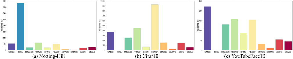
Runtime. As observed from Table 1, CICAG exhibits linear complexity in terms of the number of samples, anchors, and features. When the number of anchors and features is large, CICAG is more efficient compared to other algorithms. However, since the publicly available datasets have generally undergone preprocessing such as feature extraction or dimensionality reduction, making m and d relatively small, CICAG's efficiency advantage is not as apparent. Nevertheless, Figure 2 shows that, CICAG's efficiency consistently ranks in the top three, with only a small difference from the shortest runtime. Considering the performance shown in Table 3, CICAG's efficiency is entirely acceptable. Although CAMVC requires alternating variable optimization, each variable has a closed-form solution, significantly reducing its runtime. However, once m becomes too large, CAMVC's computational complexity grows cubically, leading to a significant decrease in efficiency.
| Metric | ACC | NMI | ARI | ACC | NMI | ARI | ACC | NMI | ARI |
|---|---|---|---|---|---|---|---|---|---|
| Dataset | 3Sources | WebKB | NUS-WIDE | ||||||
| SFMC | 71.6±0.0 | 59.9±0.0 | 50.0±0.0 | 78.2±0.0 | 28.0±0.0 | 49.0±0.0 | 10.7±0.0 | 08.2±0.0 | 01.2±0.0 |
| TBGL | 72.8±0.0 | 54.8±0.0 | 45.0±0.0 | 84.1±0.0 | 18.7±0.0 | 29.2±0.0 | 07.8±0.0 | 05.2±0.0 | 08.2±0.0 |
| FPMVS | 32.5±0.0 | 08.3±0.0 | 04.0±0.0 | 86.9±0.0 | 44.6±0.0 | 53.0±0.0 | 19.2±0.0 | 16.4±0.0 | 06.3±0.0 |
| OMSC | 37.9±0.0 | 14.2±0.0 | 08.1±0.0 | 93.0±0.0 | 52.6±0.0 | 70.4±0.0 | 18.1±0.0 | 16.1±0.0 | 05.9±0.0 |
| FMVACC | 71.0±0.0 | 62.9±0.0 | 58.3±0.0 | 93.2±0.0 | 54.3±0.0 | 71.7±0.0 | 17.8±0.0 | 15.1±0.0 | 05.9±0.0 |
| FDAGF | 72.8±0.0 | 51.8±0.0 | 51.1±0.0 | 93.3±0.0 | 53.7±0.0 | 71.0±0.0 | 16.9±0.0 | 16.3±0.0 | 04.7±0.0 |
| EMVGC | 61.0±0.0 | 35.6±0.0 | 33.0±0.0 | 93.9±0.1 | 57.8±0.0 | 73.2±0.1 | 18.2±0.3 | 17.1±0.3 | 05.6±0.1 |
| CAMVC | 73.4±2.4 | 66.8±0.6 | 66.2±1.9 | 87.5±0.0 | 30.9±0.0 | 44.9±0.0 | 19.1±0.3 | 19.7±0.3 | 06.1±0.1 |
| AEVC | 70.4±0.0 | 64.9±0.0 | 56.0±0.0 | 81.5±0.0 | 31.1±0.0 | 38.7±0.0 | 18.9±0.0 | 18.3±0.0 | 06.2±0.0 |
| CICAG | 75.2±3.8 | 65.5±3.1 | 59.9±5.7 | 95.2±0.0 | 64.8±0.0 | 78.6±0.0 | 20.5±0.4 | 19.2±0.2 | 06.3±0.2 |
| Dataset | Notting-Hill | Cifar10 | Cifar100 | ||||||
| SFMC TBGL FPMVS OMSC | 88.9±0.0 59.9±0.0 90.0±0.0 | 84.3±0.0 54.5±0.0 80.0±0.0 67.7±0.0 | 84.7±0.0 36.9±0.0 79.4±0.0 62.4±0.0 | 98.9±0.0 OM 99.0±0.0 | 96.9±0.0 OM 97.3±0.0 | 97.5±0.0 OM 97.8±0.0 | OM OM OM | OM OM OM OM | OM OM OM OM |
| 73.2±0.0 | 98.0±0.0 | OM | |||||||
| 78.6±0.0 | 95.3±0.0 | 95.7±0.0 | |||||||
| FMVACC | 69.8±0.0 | 57.0±0.0 | 99.2±0.0 | 97.9±0.0 | 98.3±0.0 | 91.7±0.0 | 98.0±0.0 | 92.1±0.0 | |
| FDAGF | 84.5±0.0 | 79.8±0.0 | 79.2±0.0 | 98.7±0.0 | 96.6±0.0 | 97.2±0.0 | 85.4±0.0 | 96.7±0.0 | 86.6±0.0 |
| EMVGC | 84.0±0.1 | 79.4±0.2 | 78.7±0.2 | 99.1±0.0 | 97.5±0.0 | 98.0±0.0 | 94.3±0.8 | 98.8±0.2 | 95.1±3.8 |
| CAMVC AEVC | 95.2±0.0 | 96.2±0.0 | 90.5±0.0 | 99.5±0.0 96.2±0.0 | 98.5±0.0 91.5±0.0 | 98.9±0.0 | 91.4±2.1 91.6±0.0 | 98.2±0.5 98.1±0.0 | 92.8±2.2 |
| 87.8±0.0 | 75.0±0.0 | 75.5±0.0 | 91.9±0.0 | 92.8±0.0 | |||||
| CICAG | 97.6±0.0 | 94.4±0.1 | 95.3±0.0 | 99.5±0.0 | 98.7±0.0 | 99.0±0.0 | 99.9±0.7 | 99.9±0.1 | 99.9±0.7 |
| Dataset | YouTubeFace10 | YouTubeFace20 | YouTubeFace50 | ||||||
| SFMC TBGL | 63.4±0.0 OM | 64.3±0.0 OM | 36.3±0.0 OM | 58.0±0.0 OM | 62.5±0.0 OM | 23.4±0.0 OM | OM OM | OM OM | OM OM |
| FPMVS | 75.0±0.0 | 78.7±0.0 | 67.1±0.0 | OM | OM | OM | OM | OM | OM |
| OMSC | 77.7±0.0 | 81.2±0.0 | 67.8±0.0 | OM | OM | OM | OM | OM | OM |
| FMVACC | 76.6±0.0 | 77.1±0.0 | 69.4±0.0 | 72.5±0.0 | 77.7±0.0 | 52.5±0.0 | 72.8±0.0 | 82.8±0.0 | 62.8±0.0 |
| FDAGF | 74.5±0.0 | 76.3±0.0 | 63.2±0.0 | 69.8±0.0 | 77.4±0.0 | 57.2±0.0 | 67.9±0.0 | 80.6±0.0 | 56.6±0.0 |
| EMVGC | 70.6±0.3 | 79.2±1.2 | 67.6±0.6 | 69.0±1.7 | 76.2±0.3 | 59.0±0.1 | 69.1±2.2 | 80.2±0.5 | 61.7±1.1 |
| CAMVC | 74.6±0.0 | 76.2±0.0 | 65.0±0.0 | 69.9±1.4 | 77.6±0.3 | 60.8±1.0 | 70.2±1.9 | 80.8±0.5 | 59.0±2.4 |
| AEVC | 75.6±0.0 | 78.2±0.0 | 68.6±0.0 | 71.9±0.0 | 75.9±0.0 | 61.0±0.0 | 72.3±0.0 | 82.8±0.0 | 63.5±0.0 |
| CICAG | 81.7±3.1 | 80.7±1.8 | 71.4±2.9 | 73.4±0.8 | 77.9±0.4 | 61.8±2.6 | 76.7±0.2 | 83.8±0.3 | 62.3±2.0 |
| D1 | D2 | D3 | D4 | D5 | D6 | D7 | D8 | D9 | |
|---|---|---|---|---|---|---|---|---|---|
| Z | 50.9 | 91.6 | 18.2 | 72.4 | 99.3 | 94.2 | 73.3 | 69.3 | 72.6 |
| Z(i) min | 41.4 | 51.4 | 12.9 | 58.9 | 84.9 | 91.3 | 69.6 | 65.5 | 66.7 |
| Z(i) max | 57.4 | 72.5 | 14.4 | 87.4 | 89.2 | 94.2 | 75.6 | 68.9 | 69.9 |
| Z(i) uf | 50.3 | 55.3 | 14.7 | 62.9 | 96.1 | 94.4 | 72.2 | 66.2 | 72.2 |
| Z(i) af | 71.0 | 93.2 | 17.8 | 78.6 | 99.2 | 91.7 | 76.6 | 72.5 | 72.8 |
| Ours | 75.2 | 95.2 | 20.5 | 97.6 | 99.5 | 99.9 | 81.7 | 73.4 | 76.7 |
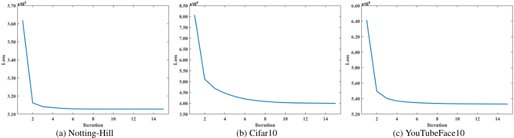
Convergence. As seen from Figure 3, the training loss of CICAG on all datasets drops rapidly at first and then stabilizes. This suggests that our algorithm not only converges but also requires only a few iterations.
4.3 Ablation Study
In Table 4, taking the D8 (YouTubeFace20) as an example: the ACC of Z, learned via Equation (2), is 69.3; the ACCs of Z(i) , learned via Equation (3), range from 65.5 to 68.9; direct fusion yields an ACC of 66.2; alignment followed by fusion achieves 72.5; and CICAG touches 73.4. These results demonstrate that simultaneously capturing both individuality and commonality is effective.
4.4 Parameter Sensitivity
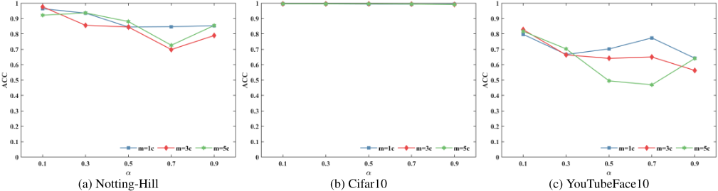
m&α. As shown in Figure 4, the trend of ACC with varying α is similar across different m, with their maximum values being close. Generally, setting m = 3c is a good choice. As α increases, the ACC of CICAG on NUS-WIDE, Cifar10, Cifar100, YouTubeFace20, and YouTubeFace50 does not show significant changes, while it exhibits a downward trend on WebKB, Notting-Hill, and YouTubeFace10, and a decrease followed by an increase on 3Sources. Overall, α achieves its maximum value around 0.1. Although the ACC at α = 0.1 is not optimal for WebKB and YouTubeFace, it is still very close to the maximum value. Therefore, setting α = 0.1 is generally a good choice.
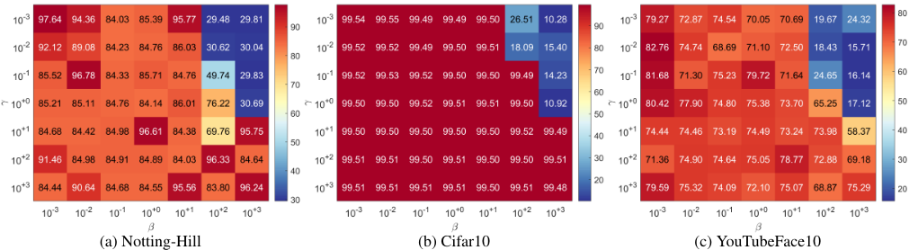
β&γ. As shown in Figure 5, β should generally not exceed γ, while γ itself is relatively insensitive. However, in pursuit of optimal values, neither should be set too high.
5 Conclusion
This paper addresses a challenge in anchor-based multi-view subspace learning. Although multiple views share the same anchor graph to capture the commonality across views, this approach clearly overlooks the individuality of specific views. As a result, some models independently explore the individuality of each view, leading to issues of alignment and fusion of anchor graphs across views. Therefore, this paper proposes a new model, capturing both the individuality and commonality of anchor graphs for multi-view clustering. The model not only allows view-specific anchor graphs to be aligned in realtime based on a common anchor graph, but also generates a balanced sample distribution and cluster-level anchors to enhance discriminative power. Moreover, it is computationally efficient in terms of sample, anchor, feature and cluster numbers. Finally, comprehensive experiments demonstrate that our model is highly competitive in terms of both effectiveness and efficiency compared to other state-of-the-art models.
Acknowledgments
This work was supported in part by the National Natural Science Foundation of China under Grants 62236001, 62276212, and 62176212.
@inproceedings{ijcai2025p652,
  title     = {Capturing Individuality and Commonality Between Anchor Graphs for Multi-View Clustering},
  author    = {Lu, Zhoumin and Yu, Yongbo and Ma, Linru and Nie, Feiping and Wang, Rong},
  booktitle = {Proceedings of the Thirty-Fourth International Joint Conference on
               Artificial Intelligence, {IJCAI-25}},
  publisher = {International Joint Conferences on Artificial Intelligence Organization},
  editor    = {James Kwok},
  pages     = {5860--5868},
  year      = {2025},
  month     = {8},
  note      = {Main Track},
  doi       = {10.24963/ijcai.2025/652},
  url       = {https://doi.org/10.24963/ijcai.2025/652},
}
TY - CPAPER TI - Capturing Individuality and Commonality Between Anchor Graphs for Multi-View Clustering AU - Lu, Zhoumin AU - Yu, Yongbo AU - Ma, Linru AU - Nie, Feiping AU - Wang, Rong T2 - Proceedings of the Thirty-Fourth International Joint Conference on Artificial Intelligence, IJCAI-25 PB - International Joint Conferences on Artificial Intelligence Organization PY - 2025 SP - 5860 EP - 5868 DO - 10.24963/ijcai.2025/652 UR - https://doi.org/10.24963/ijcai.2025/652 ER -Copied
Machine-readable versions of this paper, for tools and AI agents:





