
MCF-Spouse: A Multi-Label Causal Feature Selection Method with Optimal Spouses Discovery
Proceedings of the Thirty-Fourth International Joint Conference on Artificial Intelligence. Main Track. Pages 5914-5922.
https://doi.org/10.24963/ijcai.2025/658
Keywords
- Machine Learning: ML: Multi-label learning
- Machine Learning: ML: Causality
- Machine Learning: ML: Bayesian learning
Abstract
Multi-label causal feature selection has garnered considerable attention for its ability to identify the most informative features while accounting for the causal dependencies between labels and features. However, previous work often overlooks the unique contributions of labels to the target variables in multi-label settings, focusing instead on prioritizing feature variables. Moreover, existing methods typically rely on traditional Markov Blanket (MB) discovery to construct an initial MB, which often fails to explore the most valuable form of spouse variables to feature selection in multi-label scenarios, leading to significant computational overhead due to redundant Conditional Independence (CI) tests required for spouse search. To address these challenges, we propose the Multi-label Causal Feature Selection Method with Optimal Spouses Discovery, MCF-Spouse, which leverages mutual information to quantify the contributions of both labels and features, ensuring the retention of the most informative variables in multi-label settings. Moreover, we systematically analyzes all potential forms of spouse variables to identify the optimal spouse case, significantly reducing the spouse search space and alleviating the time overhead associated with CI tests. Experiments conducted on diverse real-world datasets demonstrate that MCF-Spouse consistently outperforms state-of-the-art methods across multiple metrics, offering a scalable and interpretable solution for multi-label causal feature selection.
- [Aliferis et al., 2003] Constantin F Aliferis, Ioannis Tsamardinos, and Alexander Statnikov. Hiton: a novel markov blanket algorithm for optimal variable selection. In AMIA annual symposium proceedings, volume 2003, page 21. American Medical Informatics Association, 2003.
- [Aliferis et al., 2010a] Constantin F Aliferis, Alexander Statnikov, Ioannis Tsamardinos, Subramani Mani, and Xenofon D Koutsoukos. Local causal and markov blan- ket induction for causal discovery and feature selection for classification part i: algorithms and empirical evaluation. Journal of Machine Learning Research, 11(1), 2010.
- [Aliferis et al., 2010b] Constantin F Aliferis, Alexander Statnikov, Ioannis Tsamardinos, Subramani Mani, and Xenofon D Koutsoukos. Local causal and markov blan- ket induction for causal discovery and feature selection for classification part ii: analysis and extensions. Journal of Machine Learning Research, 11(1), 2010.
- [Ben-Gal, 2008] Irad Ben-Gal. Bayesian networks. Encyclo- pedia of statistics in quality and reliability, 2008.
- [Cai and Zhu, 2018] Zhiling Cai and William Zhu. Multi- label feature selection via feature manifold learning and sparsity regularization. International journal of machine learning and cybernetics, 9:1321-1334, 2018.
- [Chu et al., 2023] Zhixuan Chu, Ruopeng Li, Stephen Rath- bun, and Sheng Li. Continual causal inference with in- cremental observational data. In 2023 IEEE 39th Inter- national Conference on Data Engineering (ICDE), pages 3430-3439. IEEE, 2023.
- [Elisseeff and Weston, 2001] André Elisseeff and Jason We- ston. A kernel method for multi-labelled classification. Advances in neural information processing systems, 14, 2001.
- [Faraji et al., 2024] Mohammad Faraji, Seyed Amjad Seyedi, Fardin Akhlaghian Tab, and Reza Mahmoodi. Multi-label feature selection with global and local label correlation. Expert Systems with Applications, 246:123198, 2024.
- [Gao et al., 2017] Tian Gao, Kshitij Fadnis, and Murray Campbell. Local-to-global bayesian network structure learning. In International Conference on Machine Learn- ing, pages 1193-1202. PMLR, 2017.
- [Gonc ¸alves et al., 2013] Eduardo Corrêa Gonc ¸alves, Alexandre Plastino, and Alex A Freitas. A genetic algorithm for optimizing the label ordering in multi-label classifier chains. In 2013 IEEE 25th international confer- ence on tools with artificial intelligence, pages 469-476. IEEE, 2013.
- [Gonzalez-Lopez et al., 2020] Jorge Gonzalez-Lopez, Se- bastián Ventura, and Alberto Cano. Distributed multi-label feature selection using individual mutual information mea- sures. Knowledge-Based Systems, 188:105052, 2020.
- [Guo et al., 2023] Xianjie Guo, Kui Yu, Lin Liu, Peipei Li, and Jiuyong Li. Adaptive skeleton construction for accu- rate dag learning. IEEE Transactions on Knowledge and Data Engineering, 2023.
- [Guo et al., 2024] Xianjie Guo, Kui Yu, Lin Liu, Jiuyong Li, Jiye Liang, Fuyuan Cao, and Xindong Wu. Progressive skeleton learning for effective local-to-global causal struc- ture learning. IEEE Transactions on Knowledge and Data Engineering, 2024.
- [Huang et al., 2018] Rui Huang, Weidong Jiang, and Guan- gling Sun. Manifold-based constraint laplacian score for multi-label feature selection. Pattern Recognition Letters, 112:346-352, 2018.
- [Jian et al., 2016] Ling Jian, Jundong Li, Kai Shu, and Huan Liu. Multi-label informed feature selection. In IJCAI, vol- ume 16, pages 1627-33, 2016. IJCAI
- [Kraskov et al., 2004] Alexander Kraskov, Harald Stögbauer, and Peter Grassberger. Estimating mutual information. Physical Review E-Statistical, Nonlinear, and Soft Matter Physics, 69(6):066138, 2004.
- [Lee and Kim, 2015] Jaesung Lee and Dae-Won Kim. Mu- tual information-based multi-label feature selection using interaction information. Expert Systems with Applications, 42(4):2013-2025, 2015.
- [Li et al., 2024] Yonghao Li, Liang Hu, and Wanfu Gao. Multi-label feature selection with high-sparse personalized and low-redundancy shared common features. Information Processing & Management, 61(3):103633, 2024.
- [Ling et al., 2022a] Zhaolong Ling, Bo Li, Yiwen Zhang, Qingren Wang, Kui Yu, and Xindong Wu. Causal feature selection with efficient spouses discovery. IEEE Transac- tions on Big Data, 9(2):555-568, 2022.
- [Ling et al., 2022b] Zhaolong Ling, Ying Li, Yiwen Zhang, Kui Yu, Peng Zhou, Bo Li, and Xindong Wu. A light causal feature selection approach to high-dimensional data. IEEE Transactions on Knowledge and Data Engi- neering, 2022.
- [Ling et al., 2024a] Zhaolong Ling, Bo Li, Yiwen Zhang, Peng Zhou, Xingyu Wu, Yuee Huang, Kui Yu, and Xin- dong Wu. Causal discovery using weight-based condi- tional independence test. ACM Transactions on Knowl- edge Discovery from Data, 19(1):1-24, 2024.
- [Ling et al., 2024b] Zhaolong Ling, Jingxuan Wu, Yiwen Zhang, Peng Zhou, Xingyu Wu, Kui Yu, and Xindong Wu. Label-aware causal feature selection. IEEE Transactions on Knowledge and Data Engineering, 2024.
- [Liu et al., 2020] Jinghua Liu, Yuwen Li, Wei Weng, Jia Zhang, Baihua Chen, and Shunxiang Wu. Feature selec- tion for multi-label learning with streaming label. Neuro- computing, 387:268-278, 2020.
- [Ma et al., 2012] Zhigang Ma, Feiping Nie, Yi Yang, Jasper RR Uijlings, and Nicu Sebe. Web image annotation via subspace-sparsity collaborated feature selection. IEEE Transactions on Multimedia, 14(4):1021-1030, 2012.
- [Ma et al., 2025] Lin Ma, Liang Hu, Yonghao Li, Weiping Ding, and Wanfu Gao. Mi-mcf: A mutual information- based multilabel causal feature selection. IEEE Trans- actions on Neural Networks and Learning Systems, 36(6):9864-9878, 2025.
- [Masegosa and Moral, 2012] Andrés R Masegosa and Serafín Moral. A bayesian stochastic search method for discovering markov boundaries. Knowledge-Based Systems, 35:211-223, 2012.
- [Pearl, 2014] Judea Pearl. Probabilistic reasoning in intel- ligent systems: networks of plausible inference. Elsevier, 2014.
- [Pellet and Elisseeff, 2008] Jean-Philippe Pellet and André Elisseeff. Using markov blankets for causal structure learning. Journal of Machine Learning Research, 9(7), 2008.
- [Pena et al., 2007] Jose M Pena, Roland Nilsson, Johan Björkegren, and Jesper Tegnér. Towards scalable and data efficient learning of markov boundaries. International Journal of Approximate Reasoning, 45(2):211-232, 2007.
- [Pereira et al., 2018] Rafael B Pereira, Alexandre Plastino, Bianca Zadrozny, and Luiz HC Merschmann. Categoriz- ing feature selection methods for multi-label classification. Artificial intelligence review, 49:57-78, 2018.
- [Read et al., 2008] Jesse Read, Bernhard Pfahringer, and Ge- off Holmes. Multi-label classification using ensembles of pruned sets. In 2008 eighth IEEE international conference on data mining, pages 995-1000. IEEE, 2008.
- [Shao et al., 2013] Huan Shao, GuoZheng Li, GuoPing Liu, and YiQin Wang. Symptom selection for multi-label data of inquiry diagnosis in traditional chinese medicine. Sci- ence China Information Sciences, 56:1-13, 2013.
- [Spirtes et al., 2001] Peter Spirtes, Clark Glymour, and Richard Scheines. Causation, prediction, and search. MIT press, 2001.
- [Statnikov et al., 2013] Alexander Statnikov, Nikita I Lytkin, Jan Lemeire, and Constantin F Aliferis. Algorithms for discovery of multiple markov boundaries. Journal of Ma- chine Learning Research, 14(Feb):499-566, 2013.
- [Tsamardinos et al., 2003a] Ioannis Tsamardinos, Con- stantin F Aliferis, and Alexander Statnikov. Time and sample efficient discovery of markov blankets and direct causal relations. In Proceedings of the ninth ACM SIGKDD international conference on Knowledge discovery and data mining, pages 673-678, 2003.
- [Tsamardinos et al., 2003b] Ioannis Tsamardinos, Con- stantin F Aliferis, Alexander R Statnikov, and Er Stat- nikov. Algorithms for large scale markov blanket discovery. In FLAIRS, volume 2, pages 376-81, 2003.
- [Tsamardinos et al., 2006] Ioannis Tsamardinos, Laura E Brown, and Constantin F Aliferis. The max-min hill- climbing bayesian network structure learning algorithm. Machine learning, 65:31-78, 2006.
- [Wu et al., 2020] Xingyu Wu, Bingbing Jiang, Kui Yu, Huanhuan Chen, and Chunyan Miao. Multi-label causal feature selection. In Proceedings of the AAAI conference on artificial intelligence, volume 34, pages 6430-6437, 2020.
- [Wu et al., 2022] Xingyu Wu, Bingbing Jiang, Yan Zhong, and Huanhuan Chen. Multi-target markov boundary dis- covery: Theory, algorithm, and application. IEEE Trans- actions on Pattern Analysis and Machine Intelligence, 45(4):4964-4980, 2022.
- [Wu et al., 2023a] Xingyu Wu, Bingbing Jiang, Xiangyu Wang, Taiyu Ban, and Huanhuan Chen. Feature selection in the data stream based on incremental markov bound- ary learning. IEEE Transactions on Neural Networks and Learning Systems, 34(10):6740-6754, 2023.
- [Wu et al., 2023b] Xingyu Wu, Bingbing Jiang, Tianhao Wu, and Huanhuan Chen. Practical markov boundary learning without strong assumptions. In Proceedings of the AAAI Conference on Artificial Intelligence, volume 37, pages 10388-10398, 2023.
- [Xu et al., 2016] Jianhua Xu, Jiali Liu, Jing Yin, and Chengyu Sun. A multi-label feature extraction algo- rithm via maximizing feature variance and feature-label dependence simultaneously. Knowledge-Based Systems, 98:172-184, 2016.
- [Yu et al., 2021] Kui Yu, Mingzhu Cai, Xingyu Wu, Lin Liu, and Jiuyong Li. Multilabel feature selection: a local causal structure learning approach. IEEE Transactions on Neural Networks and Learning Systems, 34(6):3044-3057, 2021.
- [Zhang and Zhou, 2007] Min-Ling Zhang and Zhi-Hua Zhou. Ml-knn: A lazy learning approach to multi-label learning. Pattern recognition, 40(7):2038-2048, 2007.
- [Zhang et al., 2019a] Jia Zhang, Zhiming Luo, Candong Li, Changen Zhou, and Shaozi Li. Manifold regularized dis- criminative feature selection for multi-label learning. Pat- tern Recognition, 95:136-150, 2019.
- [Zhang et al., 2019b] Ping Zhang, Guixia Liu, and Wanfu Gao. Distinguishing two types of labels for multi-label feature selection. Pattern recognition, 95:72-82, 2019.
- [Zhang et al., 2020] Ping Zhang, Wanfu Gao, Juncheng Hu, and Yonghao Li. Multi-label feature selection based on high-order label correlation assumption. Entropy, 22(7):797, 2020.
References were extracted automatically from the PDF and may contain errors.
Full text extracted automatically from the PDF; figures, tables and equations may differ. The PDF is the version of record.
1 Introduction
Causal inference is crucial in machine learning, enhancing model efficiency, interpretability, and predictive accuracy in complex domains [Chu et al., 2023; Ma et al., 2025]. One of the fundamental methods to causal inference involves Bayesian networks (BNs) [Ben-Gal, 2008; Pearl, 2014], which utilize directed acyclic graphs (DAGs) to
∗Corresponding author
jchu@jlu.edu.cn∗
model dependencies among variables [Aliferis et al., 2010a; Aliferis et al., 2010b]. Within a BN, the Markov blanket (MB) [Tsamardinos et al., 2003b] of a target variable captures its essential local causal structure, comprising direct causes (parents), direct effects (children), and other causes of its children (spouses). Identifying MBs across multiple variables imposes valuable constraints, effectively reducing the search space and facilitating more scalable approaches for inferring large-scale BNs [Tsamardinos et al., 2006; Pellet and Elisseeff, 2008; Gao et al., 2017]. More importantly, prior studies have demonstrated that the MB represents the optimal feature subset, as all other features become independent of the target when conditioned on its MB, which underscores its significance in feature selection applications [Masegosa and Moral, 2012; Statnikov et al., 2013].
Single-label causal feature selection methods focus on identifying relevant features for a single target variable [Ling et al., 2022b; Guo et al., 2023; Ling et al., 2024a]. These methods fail to consider label dependencies, which are essential in multi-label scenarios [Ling et al., 2024b; Guo et al., 2024]. For example, when predicting diabetes and hypertension, features such as BMI and cholesterol may influence both conditions, highlighting the interdependencies between labels. Multi-label causal feature selection addresses this issue by simultaneously capturing feature-feature, featurelabel, and label-label relationships [Wu et al., 2020; Yu et al., 2021; Wu et al., 2022]. By considering causal relationships across multiple labels, multi-label causal feature selection tries to capture the underlying structure among featurefeature, feature-label and label-label simultaneously, enhancing model performance and interpretability in multi-label settings [Yu et al., 2021].
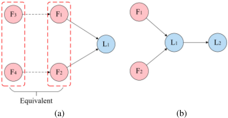
However, due to the unique characteristics of multi-label scenarios, several challenges arise in identifying the MB for target labels. First, complex interdependencies often challenge the faithfulness assumption [Pearl, 2014], particularly due to the presence of equivalent information [Wu et al., 2022]. As illustrated in Fig. 1.(a), {F1, F2} directly convey information to L1 through the paths F1 → L1 and F2 → L1. {F3, F4} have the paths to {F1, F2} as F3 → F1 and F4 → F2. In this case, {F3, F4} provide equivalent information to L1 as {F1, F2}, raising the question of which variables should be retained in L1's MB. Furthermore, as shown in Fig. 1.(b), the equivalent information provided by L1 and {F1, F2} presents additional challenges in the presence of strong correlations between labels. Specifically, L1, which encapsulates the information from {F1, F2}, can act as a blocker, obstructing the path from {F1, F2} to L2 according to the definition of D-separation [Pearl, 2014]. This complicates the identification of informative variables within the MB, as it requires careful consideration of the interplay between features and labels to avoid redundancy or loss of crucial information. Existing studies [Wu et al., 2020; Yu et al., 2021; Wu et al., 2022] tend to retain as many features as possible, prioritizing features over labels. These methods frequently recover features blocked by strong label correlations through extensive Conditional Independence (CI) tests. However, in multi-label contexts, the relationships between labels are equally critical. It is possible that labels, as output variables, encapsulate more concentrated and predictive information than input features, which primarily represent attributes. It is essential to develop methods that not only account for the equivalent information provided by features and labels but also leverage the rich interdependencies between labels to enhance the identification of the MB.
More importantly, in multi-label causal feature selection, spouse sets are crucial for capturing the complete Markov blanket of a target label by addressing indirect causal relationships [Ling et al., 2022a]. Unlike parent and children variables, which represent direct causal influences, spouse variables affect the target variables through their impact on shared children. This makes spouse variables essential for modeling the intricate interactions and dependencies among multiple labels. Ignoring spouse variables can lead to incomplete MBs, since indirect effects can be overlooked, potentially resulting in biased outcomes. The inclusion of spouse variables is particularly important in multi-label scenarios, where labels often share common causes or are connected through indirect pathways. However, researchers often overlook the spouse variables, focusing instead on PC variables, under the assumption that PC variables contain the most relevant information for the target variables [Wu et al., 2020; Yu et al., 2021]. Alternatively, some methods rely on existing MB construction such as HITON-MB [Aliferis et al.,
2003], MMMB [Tsamardinos et al., 2003a], and GetPC [Pena et al., 2007] to establish the initial MB, followed by further optimization [Wu et al., 2022; Wu et al., 2023a; Wu et al., 2023b]. These methods may either risk compromising the integrity of the MB or introduce significant CI tests due to the high dimensionality of features and labels in multi-label datasets when searching for spouse sets.
In this article, we propose the Multi-label Causal Feature Selection Method with Optimal Spouse Discovery (MCFSpouse), which addresses key challenges in multi-label causal feature selection through several innovations. First, to tackle the issues of equivalent information and the blockage of paths from features to labels caused by strong label correlations, we utilize mutual information (MI) [Zhang et al., 2019b; Pereira et al., 2018] to quantify the contributions of both labels and features to the target variable. This approach ensures that only the most informative variables are retained, prioritizing labels when they provide greater predictive value. Second, to efficiently identify spouse variables without incurring significant computational overhead from CI tests, we systematically analyze all possible configurations of spouse variables in the multi-label domain. By leveraging target-specific guidance, we pinpoint the optimal spouse variables to include in the target's Markov blanket. This targeted strategy significantly narrows the search space for spouse variables, reducing computational complexity and minimizing time overhead. The main contributions of this paper are summarized as follows:
- We discuss all the possible spouse relationships in the context of multi-label causal feature selection, and analyze the optimal spouse set through the guidance of target-specific variables.
- To solve the equivalent information and the blockage of paths from features to labels caused by strong label correlations, we use mutual information to compare the contribution of features and labels, and maintain the most informative variables.
- We conduct extensive experiments to validate our MCFSpouse method, comparing it with nine state-of-the-art multi-label feature selection methods on four metrics across eight real-world datasets. The results consistently show that our MCF-Spouse method outperforms the compared methods across all four metrics.
2 RelatedWork
Non-BN-based methods. These methods can be categorized into three categories [Pereira et al., 2018]. Mutual information-based methods, such as D2F [Lee and Kim, 2015], MCMFS [Zhang et al., 2020], ENM [Gonzalez-Lopez et al., 2020], and FSSL [Liu et al., 2020], select features by evaluating mutual information between features and labels. Regularization-based methods, including SFUS [Ma et al., 2012], MIFS [Jian et al., 2016], MLFS-GLOCAL [Faraji et al., 2024], and ESRFS [Li et al., 2024], incorporate regularization terms to enhance feature selection. Manifold learning-based methods, such as MCLS [Huang et al., 2018], MSSL [Cai and Zhu, 2018], and MDFS [Zhang et al., 2019a], exploit geometric structures within data. While these methods improve classification performance and mitigate the curse of dimensionality, they can not select the optimal number of features automatically and explicitly model feature-feature and label-label dependencies.
BN-based methods. BN-based methods offer significant advantages by simultaneously modeling feature-feature, feature-label, and label-label relationships [Yu et al., 2021]. For instance, Wu et al. explore causal mechanisms in multilabel feature selection by distinguishing common features and label-specific features in MB-MCF [Wu et al., 2020]. They further extend this work with CLFS [Wu et al., 2022], focusing on the interplay between common MB variables and equivalent information. Similarly, Yu et al. [Yu et al., 2021] address the issue of false discoveries-where A appears in the MB set of B, but B is absent from the MB set of A in M2LC. This method reduces computational complexity by learning local BN structures rather than entire BN structure.
However, existing BN-based methods often suffer from high computational overhead due to redundant CI tests during spouse discovery. Furthermore, the complex dependencies in multi-label feature selection often lead to equivalent information, making it challenging to determine the most informative MB variables. To address these issues, we propose an efficient spouse discovery method and leverage mutual information to accurately evaluate the contributions of both features and labels, thereby reducing complexity and improving feature selection performance.
3 Preliminaries
In this section, we elaborate on the fundamental definitions and theorems relevant to our discussion. Based on these, we present the theorems and provide their proofs in this article.
Definition 1 (Faithfulness [Pearl, 2014]): a Directed Acyclic Graph (DAG) G is considered faithful to the probability distribution P(V ) in the Bayesian Network < V,G, P(V ) > iff every conditional independence relationship encoded in P is implied by G and satisfies the Markov condition. Furthermore, P(V ) is deemed faithful iff G accurately represents P (V ).
Definition 2 (Equivalent information [Statnikov et al., 2013]): as illustrated in Fig. 1.(a), the features {F3, F4} provide the same information to the label L1 as {F1, F2}. This equivalence implies that {F1, F2} can be replaced by {F3, F4} without any loss of information. In this scenario, {F1, F2} and {F3, F4} are considered equivalent information in their contribution to L1.
The faithfulness condition in Definition 1 is always invalid due to the presence of equivalent information in the context of multi-label learning and raises the question of which should be retained in the target's Markov blanket. We introduce Definition 3 and 4 and Theorem 1 to solve this problem.
Definition 3 (Common causal variable): as illustrated in Fig. 2, C is identified as the common variable, since it is present in the Markov blankets of both X and Y .
Definition 4 (Target-specific variable): as illustrated in Fig. 2, A is the target-specific variable for X, and B is the target-specific variable for Y , which means that A
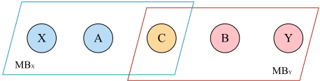
uniquely captures the local dependencies relevant to X, and B uniquely captures the local dependencies relevant to Y .
Target-specific MB variables capture the unique local relationships specific to individual targets, enabling more accurate predictions or inferences tailored to each target. In contrast, common MB variables represent shared dependencies across multiple targets, efficiently summarizing the information relevant to all targets using a minimal set of variables.
Theorem 1. Equivalent information can be resolved by comparing the contributions of a feature F and a label L2 to the target label L1.
Proof. Mutual information [Kraskov et al., 2004] is a widely used metric for evaluating the contribution of variables. In the context of feature F and labels L1 and L2, we compare the mutual information between feature F and target label L1 (I(L1; F )) with the mutual information between label L2 and target label L1 (I(L1;L2)).
If I(L1; F) ≤ I(L1;L2), this implies that feature F provides information similar to that of label L2 or is redundant. In such cases, we choose not to retain F, thereby reducing redundancy from equivalent information. Conversely, if I(L1; F) > I(L1;L2), the feature F offers additional information beyond what label L2 provides, and we therefore retain F .
Definition 5 (V-structure [Pearl, 2014]): three variables X, Y and T form a V-structure (i.e., X → T ← Y ), iff X and Y have a directed edge pointing to T, regardless of whether X and Y are directly connected.
The V-structure is a critical concept for identifying the spouse set of a variable. For example, in a V-structure T → X ← Y , Y is a spouse of T, and X is a collider. However, in the context of multi-label causal feature selection, directly applying Definition 5 for spouse search can lead to several issues: first, as the number of features and labels increases, the time overhead grows exponentially due to the need of numerous conditional independence tests; second, in the multi-label domain, the identification of spouses is more complex, as illustrated in Fig. 3, which presents four cases of spouse relationships in a multi-label DAG. It is not clear which spouse should be retained. To address these challenges, we introduce Theorem 2 for efficient and precise spouse search.
In Fig. 3, we illustrate the four possible relationships between the target label and the spouse. Based on this figure, we conclude that Fig. 3.(a) is the case we want to retain, as the spouse of L1 is the feature F3. In the case of Fig. 3.(b), we do not need to retain it since the spouse of L1 here is label L2.
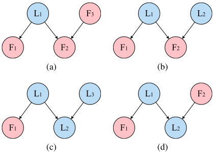
If we designate label L2 as the spouse of L1, we will conduct feature selection using only the feature set from L1's Markov blanket, making it unnecessary to retain label L2. Similarly, in Fig. 3.(c), we also do not need to retain it, since the spouse of L1 in this case is label L3. Finally, for Fig. 3.(d), we conclude that it should not be retained, as proven in Theorem 2.
Theorem 2. The label-specific variable is not contained in other label's MB.
Proof. According to Definition 4, in Fig. 3.(d), feature F2 is the label-specific variable of label L2. Therefore, the following conditions hold:
- F2 ̸⊥⊥ L2 | {L\L2}, which indicates that F2 is dependent on L2 conditioned on the rest of the label set L\L2.
- ∀L ∈ L,L ̸= L2, F2 ⊥⊥ L | {L\L2}, meaning F2 is independent of any other label L (where L ̸= L2) conditioned on L\L2.
Assume that F2 is part of the Markov blanket of label L1. This implies that there exists a path between F2 and L1, such as L1 → L2 ← F2. According to this path, F2 ̸⊥⊥ L1 | {L\L1}, indicating that F2 is dependent on L1 given the rest of the labels. However, this contradicts the earlier condition that F2 is independent of all other labels except L2.
Thus, we reach a contradiction. Therefore, F2 cannot be part of the Markov blanket of L1, and more generally, a labelspecific variable cannot be contained in the Markov blanket of any other label.
Theorem 3. For three variables X, Y and T , given condition set Z if T ̸⊥⊥ X | Z, T ⊥⊥ Y | Z, T ̸⊥⊥ Y | Z ∪X, then T, X and Y form a V-structure (T → X ← Y ), variable Y is T's spouse [Spirtes et al., 2001; Pearl, 2014].
Theorem 4. Only children with multiple parents can make target variable T and variables in non-PCT from independence to dependence [Ling et al., 2022a].
According to Theorems 2, 3, and 4, the spouse search can be conducted within a multi-label scenario. First, we identify children with multiple parents, which can serve as colliders.
Then, we determine the optimal spouse set, which is illustrated in Fig. 3.(a), indicating that spouses can only take the form of feature-feature pairs. Finally, using Theorem 3, we can estimate the existence of a spouse variable based on the identification of the V-structure.
4 MCF-Spouse Algorithm
In this section, we present the Multi-label Causal Feature Selection with Optimal Spouse Discovery (MCF-Spouse, Algorithm 1). MCF-Spouse consists of three phases: Phase 1 (lines 1-3) mines the PC sets using the HITON-PC method [Aliferis et al., 2003], Phase 2 (lines 4-17) recovers features ignored due to strong label correlation, and Phase 3 (lines 1828) conducts the spouse search.
4.1 Learning the Local Causal Structure of Each Class Label
In phase 1, we employ the HITON-PC [Aliferis et al., 2003] as our primary method for PC discovery. HITON-PC is known for its efficiency in identifying relevant features by minimizing false positives and false negatives, making it a robust choice for PC discovery in high-dimensional data. Phase 2 refers to the feature recovery. After the PC discovery in Phase 1, some features are not selected due to strong correlations between labels and the issue of equivalent information. These ignored features may still hold significant value but are overshadowed by the influence of other labels in the dataset. To address this, we re-evaluate these features to determine whether they should be included in the candidate PC set.
In lines 5-7, the feature Fj is examined. This feature does not belong to the current candidate PC set of label Li, but it could have been blocked by strong correlations with other labels, making it a candidate for recovery. Then, in lines 8-10, if Fj is dependent on Yi, Fj will be included in Fere(Yi) in descending order, and the top k1% features in Fere(Yi) are considered as the most possible ignored features. Lines 11-14 address the key condition: when label Lk is not in the condition set, feature Fj remains dependent on label Li; once label Lk is included in the condition set, feature Fj and label Li become independent. We conclude that label Lk blocks the path from Fj to Li, and this path-blocking mechanism shows how labels can obscure feature relationships, potentially leading to the omission of valuable features.
In lines 15-17, we compare the MI between feature Fj and the target label Li (I(Li; Fj)) with that between label Lk and the target label Li (I(Li;Lk)). This comparison allows us to quantify the contribution of feature Fj relative to the label Lk. If the feature Fj contributes more information to Li than label Lk, we conclude that Fj is more significant, and therefore, it is included in the candidate PC set (CPCLi ). Conversely, if label Lk provides more information than feature Fj, Lk is included in the candidate PC set instead.
4.2 Spouse Discovery
Phase 3 is spouse discovery. As discussed in Fig. 3, the optimal spouse variables can only exist in the configuration shown in Fig. 3.(a), which forms a collider structure: target → feature ← feature. In lines 19-21, we begin by traversing
Algorithm 1 MCF-Spouse Algorithm
Require: feature set F={F1, F2, . . . , Fm}, label set L={L1, L2, . . . , Ll}, PC discovery algorithm A, V =F ∪ L. Ensure: MBLi 1: {Phase 1: PC discovery using A} 2: for i = 1, ..., l do 3: CPCLi : discover the PC of Li from V \Li 4: {Phase 2: recover the ignored features caused by strong label correlation} 5: for i = 1, ..., l do 6: if ∃k ̸= i, Yk ∈ CMBYi then 7: for ∀Fj ∈ F\CMBYi do 8: if Fj ̸⊥⊥ Yi then 9: Fere(Yi) = Fere(Yi) ∪ {Fj} in descending order 10: Keep top k1% features in Fere(Yi) 11: for i = 1, ..., l do 12: if ∃k ̸= i,Lk ∈ CPCLi then 13: for ∀Fj ∈ F\CPCLi do 14: if Fj ̸⊥⊥ Li|{V \CPCLi } and Fj ⊥⊥ Li|{V \CPCLi } ∪ {Lk} then 15: if I(Li; Fj) > I(Li; Lk) then 16: CPCLi = CPCLi ∪ {Fj} 17: CPCLi = CPCLi \{Lk} 18: {Phase 3: spouse discovery} 19: for i = 1, ..., l do 20: CSPLi = ∅ 21: for ∀Fj ∈ CPCLi do 22: for p = 1, ..., m do 23: if ∃p s.t. Fj ∈ CPCp then 24: for ∀Fk ∈ {F\CPCLi } do 25: if Fk ̸⊥⊥ Li|{V \CPCLi ∪ Fj} then 26: CSPLi = CSPLi ∪ {Fk} 27: MBYi = CPCYi ∪CSPYi 28: return MBYieach feature Fj in the candidate PC set (CPCLi ). In lines 22-23, we estimate whether Fj belongs to the PC set of other features, since only features with multiple parent variables can serve as colliders. This step is crucial because identifying colliders is essential for detecting indirect dependencies between features and labels.
Then, in line 24, we define the candidate spouse set as the set of features that are not already included in CPCLi . These features have the potential to be spouses, as they are not directly connected to the target label Li but could form indirect relationships via colliders. In line 25, we determine the spouse relationship by examining the dependency between feature Fk and the target label Li when feature Fj is conditioned upon. Specifically, when Fj is part of the condition set, Fk and Li become dependent, indicating that Fk, Fj , and Li form a V-structure represented as Li → Fj ← Fk. In this V-structure, feature Fj serves as the collider, while feature Fk serves as the spouse of label Li.
Theorem 5. In a multi-label causal feature selection algorithm, employing a phased method-performing only PC set discovery in the first phase and deferring spouse discovery to the third phase, is more efficient and accurate than performing a complete MB search in the first phase.
| Datasets | Domains | Instances | Features | Labels |
|---|---|---|---|---|
| Flags | Image | 194 | 19 | 7 |
| VirusGO | Biology | 207 | 749 | 6 |
| CHD 49 | Medicine | 555 | 49 | 6 |
| PlantGO | Biology | 978 | 3091 | 12 |
| Enron | Text | 1702 | 1001 | 53 |
| Image | Image | 2000 | 294 | 5 |
| Yeast | Biology | 2417 | 103 | 14 |
| HumanGO | Biology | 3106 | 9844 | 14 |
Theorem 5 indicates that after feature recovery, spouse discovery reduces computational complexity while improving the accuracy of multi-label causal feature selection.
4.3 Complexity Analysis
The MCF-Spouse method consists of three main phases: (1) PC discovery, (2) feature recovery, and (3) spouse discovery.
Phase 1: PC Discovery: in this phase, the algorithm identifies the PC set for each label Li using a PC discovery method (e.g., HITON-PC, MMPC). The time complexity of this step is O(m · logm) for each label, where m is the number of features. Therefore, the total time complexity for this phase is O(l · m · logm), where l is the number of labels.
Phase 2: Feature Recovery: in this phase, the algorithm recovers features ignored due to strong label correlation. For each label Li, the algorithm compares the mutual information of features outside the PC set with other labels. The time complexity for this step is O(m2 l), since the MI for each feature is computed with every label.
Phase 3: Spouse Discovery: the algorithm identifies spouse features by examining V-structures in the PC set of each label. The complexity of checking dependencies and performing CI tests for each feature pair is O(m2 ) per label, resulting in a total time complexity of O(m2 l).
The overall time complexity of the MCF-Spouse algorithm is dominated by the most computationally expensive phase, which is consistent across all three phases. Consequently, the total time complexity is O(m2 l).
5 Experiment
In this experiment, we compare MCF-Spouse with nine methods, which are introduced in related work. Classification accuracy is computed using the ML-kNN [Zhang and Zhou, 2007], with the number of nearest neighbors k fixed at 10. Each experiment is repeated 10 times.
5.1 Experiment Settings
1) Datasets: we utilize eight real-world datasets sourced from various application domains, including Flags [Gonc¸alves et al., 2013], VirusGO [Xu et al., 2016], CHD 49 [Shao et al., 2013], PlantGO [Xu et al., 2016], Enron [Read et al., 2008], Image [Zhang and Zhou, 2007], Yeast [Elisseeff and Weston, 2001], and HumanGO [Xu et al., 2016] detailed in Table 1.
These datasets are accessible for download from the MultiLabel Classification Dataset Repository 1 .
- Evaluation Metrics: to assess the performance of selected feature subsets, we utilize the following four metrics in multi-label feature selection: Hamming Loss, Ranking Loss, F-micro and F-macro [Wu et al., 2020].
- Parameter Settings: for comparing methods, their parameters are set according to the suggestions in the corresponding literature. For D2F, MCMFS, ENM, and FSSL, these mutual information-based methods can not determine the optimal number of features. Therefore, we gradually increase the percentage of selected features from 1% to 20% with a step size of 1%. For SFUS, the value of α and β are searched within the range of {10-3 , 10-2 ,..., 102 , 103 }.
1 http://www.uco.es/kdis/mllresources/#3sourcesDesc
Similarly, for MDFS, the values of α, β, and γ are searched within the same range. In the case of ESRFS, the values of α, β, γ, and λ are also evaluated within {10-3 , 10-2 ,..., 102 , 103 }. Since SFUS, MDFS and ESRFS are unable to determine the optimal number of features, we incrementally increase the percentage of selected features in the same manner as mutual information-based methods.
For MB-MCF, M2LC, and MCF-Spouse, these BN-based methods do not require the number of selected features to be predetermined. However, MB-MCF and M2LC have parameters: k1 which determines the number of ignored features to be recovered, and k2, which selects the features that need to undergo symmetry checks. We perform the grid search within the range of [0.1, 1] to find the values of k1 and k2 that yield the best results. For parameter k1 in MCF-Spouse, we also perform the grid search within the range of [0.1, 1] to find the optimal performance.
| Datasets | Time(s) | |||||||||
|---|---|---|---|---|---|---|---|---|---|---|
| MCF-Spouse | M2LC | MB-MCF | D2F | MCMFS | ENM | FSSL | SFUS | MDFS | ESRFS | |
| Flags | 7.828 | 7.734 | 7.063 | 7.075 | 8.249 | 8.310 | 7.947 | 35.080 | 82.859 | 81.761 |
| Image | 137.016 | 278.250 | 345.828 | 782.446 | 658.217 | 651.289 | 649.886 | 656.092 | 680.634 | 595.777 |
5.2 Results of MCF-Spouse ComparingWith Nine Multi-Label Feature Selection Methods
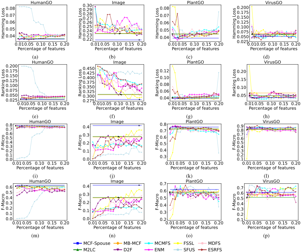
As previously discussed, Non-BN-based methods cannot determine the optimal number of features. Therefore, we incrementally increase the percentage of selected features from 1% to 20% in 1% steps to search for the optimal number. In contrast, the BN-based methods discussed in this article (MCF-Spouse, M2LC, and MB-MCF) are heuristic methods that do not require matrix training and can automatically select the optimal number of features (size of MB). These characteristics eliminate variance, further highlighting the superiority of BN-based methods. We evaluate the performance of MCF-Spouse and nine state-of-the-art methods on the HumanGO, Image, PlantGO, and VirusGO datasets. The results are shown in Fig. 4.
From Fig. 4, we observe that MCF-Spouse, which incorporates the search for spouse variables, selects more features compared to MB-MCF and M2LC-two BN-based methods that do not consider spouses. This results in significant performance improvements across the four datasets in all metrics. These findings highlight the crucial role of spouse variables in enhancing predictive accuracy and overall model performance. Compared to non-BN-based methods that determine the optimal number of features by exploring in 1% increments, MCF-Spouse consistently delivers superior performance across most datasets, with the exception of the Fmacro score on VirusGO. Non-BN-based methods often exhibit instability and require a time-intensive stepwise search to identify the optimal feature count. In contrast, MCFSpouse not only achieves more stable results but also effectively selects a smaller subset of features with higher precision, leading to better overall performance.
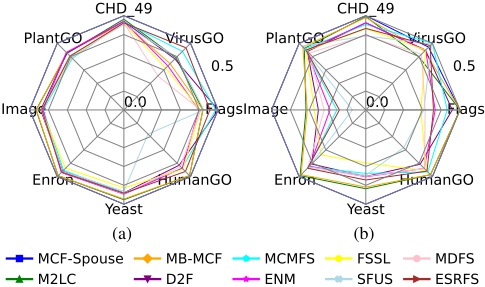
To demonstrate the stability [Wu et al., 2022] of MCFSpouse across various metrics and datasets, we normalize the results to the range [0, 0.5], assigning the best-performing method a value of 0.5. For metric Hamming Loss, lower values indicate better performance, so the minimum is normalized to 0.5. In contrast, for metric F-Macro, higher values are preferable, and the maximum is set to 0.5. As illustrated in Fig. 5, MCF-Spouse consistently demonstrates superior performance, forming a regular octagon.
5.3 Run Time Analysis
In this section, we evaluate the runtime of ten methods on the Flags and Image datasets. The timing starts at the beginning of the method and ends after classification using ML-kNN. For Non-BN-based methods, runtimes are averaged across feature selections ranging from 1% to 20% of the total features to ensure a fair comparison.
As summarized in Table 2, the proposed MCF-Spouse method demonstrates competitive efficiency. On the Flags dataset, its runtime is comparable to methods like MCMFS and ENM. For the larger Image dataset, MCF-Spouse significantly reduces runtime compared to MB-MCF, MCMFS, and others. These results highlight MCF-Spouse's ability to maintain a favorable balance between computational efficiency and feature selection quality, making it highly applicable for complex, high-dimensional datasets.
6 Conclusion
In this paper, we propose Multi-label Causal Feature Selection Method with Optimal Spouses Discovery (MCF-Spouse) to address challenges in multi-label causal feature selection. MCF-Spouse utilizes MI to evaluate contributions of features and labels and retain only the most informative variables, resolving issues of equivalent information and strong label correlations. Additionally, MCF-Spouse introduces a novel spouse discovery mechanism, optimizing spouse discovery through reducing search space and alleviating time overhead associated with CI tests. Our results highlight the importance of distinguishing label-label interactions and labelfeature contributions in multi-label causal inference. Future work will focus on addressing spurious variables in the MB, specifically by exploring the use of "AND" and "OR" rules to refine MB construction, further improving the accuracy and efficiency of multi-label causal feature selection.
Acknowledgments
This work is supported by the National Key Research and Development Program, Unified Integrated Development technology of scientific computing language and engineering physics modeling language[Grant No.2024YFB3310202], and by the talent project of Department of Science and Technology of Jilin Province of China[Grant No.20240602106RC].
@inproceedings{ijcai2025p658,
  title     = {MCF-Spouse: A Multi-Label Causal Feature Selection Method with Optimal Spouses Discovery},
  author    = {Ma, Lin and Hu, Liang and Huang, Qiang and Hao, Pingting and Hu, Juncheng},
  booktitle = {Proceedings of the Thirty-Fourth International Joint Conference on
               Artificial Intelligence, {IJCAI-25}},
  publisher = {International Joint Conferences on Artificial Intelligence Organization},
  editor    = {James Kwok},
  pages     = {5914--5922},
  year      = {2025},
  month     = {8},
  note      = {Main Track},
  doi       = {10.24963/ijcai.2025/658},
  url       = {https://doi.org/10.24963/ijcai.2025/658},
}
TY - CPAPER TI - MCF-Spouse: A Multi-Label Causal Feature Selection Method with Optimal Spouses Discovery AU - Ma, Lin AU - Hu, Liang AU - Huang, Qiang AU - Hao, Pingting AU - Hu, Juncheng T2 - Proceedings of the Thirty-Fourth International Joint Conference on Artificial Intelligence, IJCAI-25 PB - International Joint Conferences on Artificial Intelligence Organization PY - 2025 SP - 5914 EP - 5922 DO - 10.24963/ijcai.2025/658 UR - https://doi.org/10.24963/ijcai.2025/658 ER -Copied
Machine-readable versions of this paper, for tools and AI agents:





