
LLM-TPF: Multiscale Temporal Periodicity-Semantic Fusion LLMs for Time Series Forecasting
Proceedings of the Thirty-Fourth International Joint Conference on Artificial Intelligence. Main Track. Pages 6030-6038.
https://doi.org/10.24963/ijcai.2025/671
Keywords
- Machine Learning: ML: Multi-modal learning
- Machine Learning: ML: Time series and data streams
- Natural Language Processing: NLP: Language models
Abstract
Large language models have demonstrated remarkable generalization capabilities and strong performance across various fields. Recent research has highlighted their significant potential in time series forecasting. However, time series data often exhibit complex periodic characteristics, posing a substantial challenge in enabling these models to effectively capture latent patterns. To address this challenge, we propose a novel framework, LLM-TPF, which leverages individuality and commonality fusion to enhance time series forecasting. In the frequency domain, periodic features are extracted to reveal the intrinsic periodicity of the data, while textual prototypes are used to indicate temporal trends. In the time domain, carefully designed prompts are employed to guide the models in comprehending global information. A commonality fusion mechanism further aggregates heterogeneous information across dimensions, and three distinct language models are utilized to independently process different types of information. Extensive real-world experiments demonstrate that LLM-TPF is a powerful tool for time series forecasting, achieving superior performance compared to state-of-the-art specialized models and exhibiting exceptional generalization ability in zero-shot scenarios. Code is available at https://github.com/switchsky/LLM-TPF.
- [Cao et al., 2024] Defu Cao, Furong Jia, Sercan O Arik, Tomas Pfister, Yixiang Zheng, Wen Ye, and Yan Liu. TEMPO: Prompt-based generative pre-trained transformer for time series forecasting. In ICLR, 2024.
- [Copiaco et al., 2023] Abigail Copiaco, Yassine Himeur, Abbes Amira, Wathiq Mansoor, Fodil Fadli, Shadi Atalla, and Shahab Saquib Sohail. An innovative deep anomaly detection of building energy consumption using energy time-series images. Engineering Applications of Artificial Intelligence, 119:105775, 2023.
- [Hu et al., 2022] Edward J Hu, Yelong Shen, Phillip Wallis, Zeyuan Allen-Zhu, Yuanzhi Li, Shean Wang, Lu Wang, and Weizhu Chen. LoRA: Low-rank adaptation of large language models. In ICLR, 2022.
- [Huang et al., 2023] Yiming Huang, Ziyu Zhou, Zihao Wang, Xiaoying Zhi, and Xiliang Liu. Timesnet-pm2. 5: Interpretable timesnet for disentangling intraperiod and interperiod variations in pm2. 5 prediction. Atmosphere, 14(11):1604, 2023.
- [Jin et al., 2024] Ming Jin, Shiyu Wang, Lintao Ma, Zhix- uan Chu, James Y Zhang, Xiaoming Shi, Pin-Yu Chen, Yuxuan Liang, Yuan-Fang Li, Shirui Pan, and Qingsong Wen. Time-LLM: Time series forecasting by reprogram- ming large language models. In ICLR, 2024.
- [Li et al., 2024] Lulin Li, Ben Chen, Xuechao Zou, Junliang Xing, and Pin Tao. Uv-mamba: A dcn-enhanced state space model for urban village boundary identification in high-resolution remote sensing images. arXiv preprint arXiv:2409.03431, 2024.
- [Lin et al., 2024] Shengsheng Lin, Weiwei Lin, Xinyi Hu, Wentai Wu, Ruichao Mo, and Haocheng Zhong. Cyclenet: Enhancing time series forecasting through modeling peri- odic patterns. In NeurIPS, 2024.
- [Liu et al., 2023a] Haotian Liu, Chunyuan Li, Qingyang Wu, and Yong Jae Lee. Visual instruction tuning, 2023.
- [Liu et al., 2023b] Pengfei Liu, Weizhe Yuan, Jinlan Fu, Zhengbao Jiang, Hiroaki Hayashi, and Graham Neubig. Pre-train, prompt, and predict: A systematic survey of prompting methods in natural language processing. CSUR, 55(9):1-35, 2023.
- [Liu et al., 2024] Yong Liu, Tengge Hu, Haoran Zhang, Haixu Wu, Shiyu Wang, Lintao Ma, and Mingsheng Long. itransformer: Inverted transformers are effective for time series forecasting. In ICLR, 2024.
- [Liu et al., 2025] Peiyuan Liu, Hang Guo, Tao Dai, Naiqi Li, Jigang Bao, Xudong Ren, Yong Jiang, and Shu-Tao Xia. Calf: Aligning llms for time series forecasting via cross- modal fine-tuning. In AAAI, 2025.
- [Maiti et al., 2023] Abhisek Maiti, Sander Oude Elberink, and George Vosselman. Transfusion: Multi-modal fu- sion network for semantic segmentation. In CVPR, pages 6537-6547, 2023.
- [Medina-Salgado et al., 2022] Boris Medina-Salgado, Eddy Sánchez-DelaCruz, Pilar Pozos-Parra, and Javier E Sierra. Urban traffic flow prediction techniques: A review. Sus- tainable Computing: Informatics and Systems, 35:100739, 2022.
- [Nie et al., 2023] Yuqi Nie, Nam H. Nguyen, Phanwadee Sinthong, and Jayant Kalagnanam. A time series is worth 64 words: Long-term forecasting with transformers. In ICLR, 2023.
- [Pan et al., 2024] Zijie Pan, Yushan Jiang, Sahil Garg, An- derson Schneider, Yuriy Nevmyvaka, and Dongjin Song. S 2 IP-LLM:semantic space informed prompt learning with llm for time series forecasting. In ICML, 2024.
- [Radford et al., 2019] Alec Radford, Jeff Wu, Rewon Child, David Luan, Dario Amodei, and Ilya Sutskever. Language models are unsupervised multitask learners. 2019.
- [Radford et al., 2021] Alec Radford, Jong Wook Kim, Chris Hallacy, Aditya Ramesh, Gabriel Goh, Sandhini Agar- wal, Girish Sastry, Amanda Askell, Pamela Mishkin, Jack Clark, et al. Learning transferable visual models from nat- ural language supervision. In ICML, pages 8748-8763, 2021.
- [Satpute et al., 2024] Ankit Satpute, Noah Gießing, André Greiner-Petter, Moritz Schubotz, Olaf Teschke, Akiko Aizawa, and Bela Gipp. Can llms master math? inves- tigating large language models on math stack exchange. In SIGIR, pages 2316-2320, 2024.
- [Tian Zhou, 2023] Xue Wang Liang Sun Rong Jin Tian Zhou, Peisong Niu. One Fits All: Power gen- eral time series analysis by pretrained lm. In NeurIPS, 2023.
- [Wu et al., 2021a] Haixu Wu, Jiehui Xu, Jianmin Wang, and Mingsheng Long. Autoformer: Decomposition transform- ers with auto-correlation for long-term series forecasting. In NeurIPS, volume 34, pages 22419-22430, 2021.
- [Wu et al., 2021b] Yang Wu, Zijie Lin, Yanyan Zhao, Bing Qin, and Li-Nan Zhu. A text-centered shared-private framework via cross-modal prediction for multimodal sen- timent analysis. In ACL, pages 4730-4738, 2021.
- [Wu et al., 2023] Haixu Wu, Tengge Hu, Yong Liu, Hang Zhou, Jianmin Wang, and Mingsheng Long. Timesnet: Temporal 2d-variation modeling for general time series analysis. In ICLR, 2023.
- [Zeng et al., 2023] Ailing Zeng, Muxi Chen, Lei Zhang, and Qiang Xu. Are transformers effective for time series fore- casting? In AAAI, volume 37, pages 11121-11128, 2023.
- [Zhao et al., 2023] Wayne Xin Zhao, Kun Zhou, Junyi Li, Tianyi Tang, Xiaolei Wang, Yupeng Hou, Yingqian Min, Beichen Zhang, Junjie Zhang, Zican Dong, et al. A survey of large language models. arXiv preprint arXiv:2303.18223, 2023.
- [Zhou et al., 2022] Tian Zhou, Ziqing Ma, Qingsong Wen, Xue Wang, Liang Sun, and Rong Jin. Fedformer: Fre- quency enhanced decomposed transformer for long-term series forecasting. In ICML, pages 27268-27286, 2022.
References were extracted automatically from the PDF and may contain errors.
Full text extracted automatically from the PDF; figures, tables and equations may differ. The PDF is the version of record.
1 Introduction
Time series forecasting holds a pivotal position in data science and machine learning as a critical technique for analyzing and predicting data patterns that evolve over time. It finds widespread applications across various domains, such as power system load prediction in energy sectors [Copiaco et al., 2023], climate weather modeling [Huang et al., 2023], and traffic flow analysis [Medina-Salgado et al., 2022]. In recent years, pre-trained large language models (LLMs) have demonstrated remarkable potential across multiple fields, especially excelling in few-shot and even zero-shot tasks [Zhao et al., 2023].
∗Xiangjie Kong is the corresponding author.
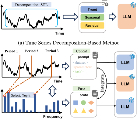
Figure 1: Difference between our approach and other integrations with LLMs. (a) Simply decomposing time series data leaves LLMs incapable of effectively understanding the periodic characteristics of the data. (b) Our approach, by integrating textual information (including prompts and textual prototypes) with time series information.
Given that both time series and textual data share sequential characteristics, leveraging the strengths of LLMs in time series forecasting is a logical and promising direction. Numerous successful cases have already validated the efficacy of LLMs in this domain. For instance, [Tian Zhou, 2023] proposed a unified framework based on pre-trained language models, achieving significant performance improvements in various time series analysis tasks and laying a solid foundation for future research. TIME-LLM [Jin et al., 2024] enriched the semantic representation of time series data through reprogramming, while CALF [Liu et al., 2025] addressed the differences between text and time series data by processing these two modalities through separate branches, thus optimizing performance. Despite achieving impressive performance in time series forecasting, the aforementioned methods still exhibit notable limitations. In particular, they fail to consider the periodic characteristics inherent in time series data (e.g., the Electricity dataset demonstrates clear seasonality and daily cycles). As shown in Figure 1, S 2 IP-LLM [Pan et al., 2024] and TEMPO [Cao et al., 2024] incorporate trend decomposition to integrate time series data into large language models. However, since large language models are primarily trained on textual data, their ability to understand and model the periodic characteristics of time series remains limited.
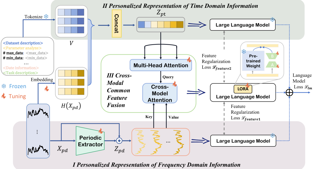
To address these issues, we propose LLM-TPF, a pretrained LLM-based time series forecasting framework that explores how to extract temporal periodic information at different scales and bridge the gap between periodic features and the semantics of LLMs by integrating personalized and common feature fusion. To overcome the difficulty that LLMs face in interpreting periodic patterns in time series data, we propose the Personalized Frequency Domain Representation (PFD) module. This module extends time series data in the frequency domain and, by integrating refined textual prototypes, captures periodic features across different frequency ranges, thereby assisting the model in better grasping longterm trends and short-term fluctuations. Given the difficulty in capturing external information in time series, we further propose the Personalized Time Domain Representation (PTD) module, which uses carefully designed prompts to guide LLMs in perceiving and integrating external features, thereby generating time-domain representations with richer contextual semantics. Finally, to address potential redundancy or conflicts between frequency and time domain features, we design the Cross-Modal Common Feature Fusion (CMF) module, which efficiently integrates and extracts common representations from both feature types through a crossmodal attention mechanism. This fully leverages the advantages of multi-source features and significantly enhances the model's forecasting performance.
In summary, the contributions of our paper can be summarized as follows:
- We propose a novel framework named LLM-TPF that enhances semantic information by integrating the periodic characteristics of time series data. To the best of our knowledge, this is the first approach to address the integration of frequency and time domain understanding within large language models for time series analysis.
- The three proposed modules integrate temporal periodic information from the frequency domain and external information from the time domain. By freezing or finetuning the large language model, these modules effectively uncover latent features in time series data, enhancing its comprehension and modeling capabilities.
- Extensive experiments are conducted on seven realworld datasets, demonstrating that LLM-TPF achieves state-of-the-art performance in both long-term and short-term time series forecasting tasks. These results validate the effectiveness and practicality of our proposed method.
2 RelatedWork
2.1 Temporal Periodicity Analysis in Time Series
Latent features such as periodicity play a crucial role in improving the prediction accuracy of time series data. For instance, Autoformer [Wu et al., 2021a] employs adaptive decomposition to separate trends and seasonal components, while FEDformer [Zhou et al., 2022] enhances long-term forecasting using frequency-domain transformations. TimesNet [Wu et al., 2023] further captures periodic features by transforming time series into a 2D frequency-domain representation, integrating multi-scale temporal and frequency information. The latest breakthrough, CycleNet [Lin et al., 2024], explicitly models the periodic characteristics of data, achieving state-of-the-art performance across multiple domains using simple linear layers or shallowMLPs. Although numerous methods exist for extracting latent periodic features from time series data, such information remains challenging for large language models to comprehend effectively.
2.2 Time Series Forecasting Using LLMs
With the rise of LLMs, an increasing number of researchers have attempted to apply them to the field of time series forecasting. Tian Zhou and colleagues pioneered the integration of pretrained large models into time series prediction [Tian Zhou, 2023], designing adapter modules tailored for various downstream tasks, thereby enabling efficient transfer and application of LLMs in this domain. Following this, many researchers further explored prompt optimization strategies. For instance, TIME-LLM [Jin et al., 2024] reformulates time series data into text-like representations more suitable for LLM processing, while CALF [Liu et al., 2025] independently processes textual and time series data, employing sophisticated modules to bridge the gap between modalities.In contrast, models like S 2 IP-LLM [Pan et al., 2024] and TEMPO [Cao et al., 2024] analyze latent periodic features within time series data and incorporate them into LLMs. However, current research has yet to fully exploit the periodic characteristics of time series data and lacks in-depth analysis across multiple scales.
2.3 Cross-modal Information Integration
Traditional multimodal fusion methods primarily focus on integrating data from different modalities. For instance, CLIP [Radford et al., 2021] employs a dual-encoder to encode text and images separately, achieving cross-modal understanding via contrastive learning, while TCSP [Wu et al., 2021b] enhances inter-modality interaction by optimizing modality fusion during feature extraction. In semantic segmentation, [Maiti et al., 2023] introduces a framework tailored to specific scenarios, minimizing lossy preprocessing and boosting fusion efficiency. At the same time, UV-Mamba [Li et al., 2024] utilizes deformable convolution networks to suppress state-space models and integrates multimodal features at the model level, fully leveraging the strengths of multiple models. Additionally, LLaVA [Liu et al., 2023a] aligns segmented image data with prompt-based inputs and trains them using large language models. These studies provide valuable insights into exploring the integration of time-series data with large language models.
3 Methodology
3.1 ProblemDefinition
In traditional time series forecasting tasks, the dynamic features at time t can be represented as Xt = (xt,1, xt,2, · · · , xt,N)⊤ ∈ RN×C , where xt,c is the feature vector of the c-th variable at time t, and C denotes the dimension of the feature variables. Additionally, we introduce a text prompt V to guide a large model in generating more precise time series forecasts. Specifically, V ∈ RL×D serves as the input prompt, where L represents the prompt length and D represents its dimensionality. Therefore, the time series forecasting problem can be simplified as follows: given the feature matrix of the past Tk time steps and the prompt information, predict the feature matrix for the next Tp time steps. This problem can be formalized as:
where Xt-Tk+1:t ∈ RTk×N×C represents the feature matrix of the past Tk time steps, V ∈ RL×D is the prompt matrix, and Xt+1:t+Tp ∈ RTp×N×C denotes the predicted feature matrix for the next Tp time steps.
3.2 Overall Architecture
Figure 2 shows the architecture of LLM-TPF, comprising threemodules: the Personalized Representation of Frequency Domain (PFD), the Personalized Representation of Time Domain (PTD), and the Cross-Modal Common Feature Fusion (CMF). The PFD extracts periodic features, while the PTD generates personalized representations using prompt tokens [Jin et al., 2024]. These features are fused by the CMF and decoded by a large language model, facilitating alignment and information sharing across modalities for better temporal and semantic modeling.
3.3 PFDModule
Frequency Domain Analysis
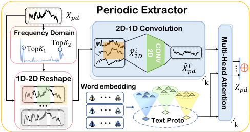
Traditional STL decomposition struggles with multi-scale and long-period time series. To address this, we use Fast Fourier Transform (FFT) to decompose the time series in the frequency domain, enabling effective analysis of different frequency components, as shown in Figure 3.
For a univariate time series Xpd ∈ RT×C , its frequency domain representation is defined as:
where FFT(·) represents the Fast Fourier Transform, and Aj denotes the weighted absolute amplitude at frequency fj, highlighting the significance of the periodic components. We apply a softmax function with a temperature parameter τ to convert amplitudes into a probability distribution, allowing us to prioritize the most significant frequencies. Specifically, the top-k frequencies {f1, . . . , fk} are selected based on the highest probabilities P(f ∗ ), where f ∗ ∈ {1, . . . , ⌊T/2⌋}. The probability P(fj) is calculated as:
Due to the ability of 2D convolution to capture periodic characteristics at different scales [Wu et al., 2023], effectively handling both long-term and short-term patterns, we adopt 2D convolution to reconstruct the time series into a 2D structure for aligning with periodic patterns and extracting temporal features:
Here, ˆXi2D represents the padded and reshaped input with dimensions pi × fi, where pi and fi are the selected period and frequency, respectively. The Conv2D operation extracts multi-scale periodic features, which are reshaped back into 1D as ˆXipd .
Text Prototype Fusion
To address the challenge of accurately representing frequency-domain temporal information in large language models, we introduce PCA-based text prototype modeling method. By applying PCA to the vocabulary embedding matrix A ∈ RV ×D , we compress it into a lower-dimensional text prototype E ∈ RV ′×D :
PCA focuses on retaining key components during dimensionality reduction, highlighting periodic and seasonal features while eliminating redundant noise. Subsequently, we fuse the temporal features ˆXipd with the text prototype E using a linear transformation and multi-head cross-attention mechanism to capture their deep associations:
Here, WX and bX are learnable parameters, and Zpd represents the aggregated periodic representation. The multihead attention mechanism enables fine-grained fusion between temporal features and textual semantics, enriching the expression of periodic information. For example, when the time series data shows an upward trend over a specific period, it can be semantically represented as "growth" or "expansion" through text descriptions.
3.4 PTDModule
Prompts play a crucial role in generative AI models, serving as guides to steer the generation of desired outputs [Liu et al., 2023b]. In the context of time-domain data, prompts can effectively assist large language models in capturing temporal information, thereby enhancing their prediction accuracy. To leverage this, we introduce time series data Xpd ∈ RT×C , which is projected into the textual semantic space through a projection function H(·). The resulting representation is then concatenated with the prompt V ∈ RL×P , creating a personalized prompt representation. This process is formalized as follows:
Where Zpt ∈ R(L+T )×D represents the concatenated personalized prompt representation, and H(Xpd) ∈ RT×D denotes the projected time series representation. Clear and precise prompts are essential for guiding large language models. We divide prompt construction into four components:
- Summarizing the dataset in natural language;
- Analyzing batch-specific parameters;
- Incorporating temporal segmentation and date information;
- Specifying task instructions.
Unlike [Jin et al., 2024], which relies on batch statistics, our approach focuses on temporal segmentation and date factors, avoiding pattern traps [Satpute et al., 2024]. This integration leverages the general knowledge of LLMs to infer deeper temporal insights, such as distinguishing between peak and off-peak electricity demand.
3.5 CMFModules
Temporal information in the frequency and time domains represents two distinct modalities with significant differences. Drawing inspiration from the interactive fusion of individual and shared features across modalities, as explored in [Wu et al., 2021b] for natural language and other modal data, we map these modalities into a unified feature space to learn a cohesive representation. Specifically, Zpt is modeled using a multi-head self-attention mechanism to effectively capture interdependencies among the elements. The resulting fused representation, ˆ Zpt, is computed as follows:
Here, WQ, WK, and WV are linear projection matrices that map the concatenated features into the attention space. This mechanism enhances cross-modal interactions and enables more accurate representation of temporal patterns. After obtaining the fused feature representation ˆ Zpt, redundant information may still persist. To refine cross-modal feature fusion, ˆ Zpt is sparsified to remove redundancy before being processed alongside the frequency-domain representation ˆ Zpd using the cross-modal attention mechanism (XMA). XMA compensates for missing periodicity and trends, producing a shared representation of the two modalities. The process is defined as:
Here, Zsh represents the shared representation between the temporal data and the prompts, achieving efficient crossmodal feature integration by fusing critical information from different modalities.
3.6 Fine-Tuning Strategy and Loss Design
We have designed differentiated fine-tuning strategies for different LLMs to better accommodate the needs of personalized and generalized representations. For personalized representations, since personalized data often contains domain-specific details that do not require frequent updates, we choose to freeze the parameters of components handling personalized representations. This approach reduces computational overhead during training while preserving the model's original semantic understanding capabilities. For generalized representations, given their cross-domain nature and the need to adapt to diverse semantic environments, we employ LowRank Adaptation [Hu et al., 2022] to achieve lightweight finetuning.
To ensure training stability and balance between personalized and generalized representations, we designed a threebranch guiding mechanism and introduced a feature regularization loss. The feature regularization loss is defined as:
The outputs Y i pd , Y i pt , and Y i sh represent the features from the i-th Transformer block for the PFD (pd), PTD (pt), and CMF (sh) modules. Here, φbi (·) applies transformations to branch b, γ (L-i) assigns layer-specific weights, and sim(·, ·) measures feature similarity to encourage alignment. The total loss is defined as:Ltotal = λ1Lfeature + λ2Llm. (12)
where Lfeature is the feature alignment loss and Llm represents the label alignment loss for multi-task learning. The weights λ1 and λ2 control the contribution of each loss term, with λ2 ≫ λ1 to prioritize task label alignment.
4 Experiments
In this section, we comprehensively evaluate our model on various benchmark datasets covering long-term, short-term, and zero-shot forecasting tasks. We also analyze the model's design and present experimental results demonstrating its effectiveness and robustness across different scenarios.
4.1 Experimental Setup
Datasets. We will perform our experiments on eight diverse datasets from different domains with broad application contexts. For long-term forecasting, we utilize the ETT series with its four subsets (ETTh1, ETTh2, ETTm1, ETTm2), along with Weather, Traffic, and Electricity datasets, same as [Wu et al., 2021a]. For short-term forecasting, we employ the M4 dataset, which includes marketing data spanning various years, quarters, and months.
Baseline. We conduct experiments with a selection of representative baseline models from recent years. These models can be categorized into four main types: (1) LLMbased methods: including Time-LLM [Jin et al., 2024], OFA [Tian Zhou, 2023] and GPT-2 [Radford et al., 2019]; (2) Transformer-based methods: including iTransformer [Liu et al., 2024] and PatchTST [Nie et al., 2023]; (3) CNN-based methods: including TimesNet [Wu et al., 2023]; (4) Linear model-based methods: including DLinear [Zeng et al., 2023].
Implementation Details. The experiments are performed on an NVIDIA RTX 3090 GPU with 24GB of memory. The Adam optimizer is employed to minimize the L1 loss, with the learning rate fixed at values within the set {1×10⁻³ , 5× 10⁻⁴ , 1 × 10⁻⁴ }. The large language model uses GPT-2 as the base model and employs LoRA for fine-tuning the large language model. A random seed of 2021 is used consistently throughout all experiments to ensure reproducibility.
4.2 Long-term and Short-termForecasting
Long-term Forecasting
Table 1 highlights the significant superiority of LLM-TPF in long-term forecasting. As observed, our proposed model outperforms all baselines in most scenarios, particularly excelling on the ETT and Electricity datasets. TIME-LLM, a recent work, was the first to introduce the reprogramming of textual prototypes. Compared to TIME-LLM and TimesNet, we observed a 4% and 18% degradation in overall performance (measured by MAE) on the ETTh2 dataset, respectively. On the multivariate Electricity dataset, our model's performance dropped by 10% compared to another SOTA model, iTransformer. Nevertheless, these results underscore the notable advantages of our model in effectively handling multivariate and periodic data.
Short-term Forecasting
Our experimental results, which are presented in Table 2, demonstrate that our method outperforms other baselines on 80% of the evaluation metrics and achieves a 5.6% overall improvement compared to the state-of-the-art TIME-LLM. This advantage is likely due to our method's consideration of feature patterns across different time series scales.
4.3 Zero-shot Learning
Compared to traditional time series forecasting models, large language model-driven frameworks are expected to demonstrate zero-shot prediction capabilities. Specifically, a model optimized on a dataset X should exhibit strong predictive performance on an unseen target dataset Y , without requiring any prior exposure to samples from Y . As shown in Table 3, we compare our proposed model with four baseline large language model-driven frameworks. Our model consistently outperforms the baselines in most scenarios. For instance, our approach achieves a reduction of 6.2% and 5.1% in error rates across all datasets compared to TIME-LLM and OFA, respectively. These results validate the effectiveness of our three-channel large language model design, which enables robust predictions without the need for task-specific training samples.
| Categories | LLM-based | Transformer-based | CNN-based | Linear-based | |||||||||||||
|---|---|---|---|---|---|---|---|---|---|---|---|---|---|---|---|---|---|
| Models Metrics | LLM-TPF MSE MAE | TIME-LLM MSE MAE | OFA MSE MAE | GPT-2 MSE MAE | iTransformer MSE MAE | PatchTST MSE MAE | TimesNet MSE MAE | Dlinear MSE MAE | |||||||||
| 96 | 0.368 | 0.386 | 0.383 | 0.412 | 0.379 | 0.402 | 0.422 | 0.428 | 0.386 | 0.405 | 0.385 | 0.408 | 0.384 | 0.402 | 0.386 | 0.400 | |
| 192 | 0.421 | 0.418 | 0.408 | 0.435 | 0.415 | 0.424 | 0.466 | 0.450 | 0.441 | 0.436 | 0.431 | 0.432 | 0.436 | 0.429 | 0.437 | 0.432 | |
| ETTh1 336 | 0.425 | 0.429 | 0.426 | 0.443 | 0.435 | 0.440 | 0.488 | 0.464 | 0.487 | 0.458 | 0.485 | 0.462 | 0.491 | 0.469 | 0.481 | 0.459 | |
| 720 | 0.451 | 0.455 | 0.443 | 0.463 | 0.441 | 0.459 | 0.485 | 0.478 | 0.503 | 0.491 | 0.497 | 0.483 | 0.521 | 0.500 | 0.519 | 0.516 | |
| 96 | 0.271 | 0.326 | 0.297 | 0.357 | 0.289 | 0.347 | 0.318 | 0.368 | 0.297 | 0.349 | 0.343 | 0.376 | 0.340 | 0.374 | 0.309 | 0.359 | |
| 192 | 0.343 | 0.373 | 0.349 | 0.390 | 0.358 | 0.392 | 0.383 | 0.407 | 0.380 | 0.400 | 0.405 | 0.417 | 0.402 | 0.414 | 0.390 | 0.406 | |
| ETTh2 336 | 0.350 | 0.387 | 0.373 | 0.408 | 0.383 | 0.414 | 0.406 | 0.427 | 0.428 | 0.432 | 0.448 | 0.453 | 0.452 | 0.452 | 0.426 | 0.444 | |
| 720 | 0.398 | 0.422 | 0.400 | 0.436 | 0.438 | 0.456 | 0.420 | 0.446 | 0.427 | 0.445 | 0.464 | 0.483 | 0.462 | 0.468 | 0.445 | 0.464 | |
| 96 | 0.283 | 0.343 | 0.291 | 0.346 | 0.296 | 0.353 | 0.330 | 0.372 | 0.334 | 0.368 | 0.339 | 0.377 | 0.338 | 0.375 | 0.335 | 0.372 | |
| 192 | 0.321 | 0.372 | 0.336 | 0.375 | 0.335 | 0.373 | 0.371 | 0.394 | 0.377 | 0.391 | 0.376 | 0.392 | 0.374 | 0.387 | 0.372 | 0.387 | |
| ETTm1 336 720 | 0.353 0.405 | 0.381 0.417 | 0.362 0.410 | 0.390 0.421 | 0.369 0.418 | 0.394 0.424 | 0.398 0.454 | 0.409 0.440 | 0.426 0.491 | 0.420 0.459 | 0.408 0.499 | 0.417 0.461 | 0.410 0.478 | 0.411 0.450 | 0.403 0.461 | 0.411 0.442 | |
| 0.310 | 0.249 | ||||||||||||||||
| 96 | 0.173 | 0.251 | 0.184 | 0.275 | 0.174 | 0.265 | 0.192 | 0.281 | 0.180 | 0.264 | 0.192 | 0.273 | 0.187 | 0.267 | 0.176 | 0.266 | |
| 192 | 0.235 | 0.295 | 0.238 | 0.231 | 0.306 | 0.245 | 0.317 | 0.250 | 0.309 | 0.252 | 0.314 | 0.309 | 0.240 | 0.307 | |||
| ETTm2 336 | 0.275 | 0.334 | 0.286 | 0.340 | 0.280 | 0.339 | 0.302 | 0.352 | 0.311 | 0.348 | 0.318 | 0.357 | 0.321 | 0.351 | 0.304 | 0.345 | |
| 720 96 | 0.361 0.153 | 0.387 0.207 | 0.379 | 0.403 0.210 | 0.373 | 0.402 | 0.399 | 0.408 | 0.412 0.174 | 0.407 0.214 | 0.413 0.171 | 0.416 0.230 | 0.408 0.172 | 0.403 0.251 | 0.406 0.159 | 0.400 0.218 | |
| 192 | 0.201 | 0.247 | 0.158 0.197 | 0.245 | 0.162 0.204 | 0.212 0.248 | 0.181 0.222 | 0.232 0.266 | 0.221 | 0.254 | 0.219 | 0.271 | 0.219 | 0.279 | 0.211 | 0.266 | |
| 720 | 0.318 | 0.342 | 0.319 | 0.326 | 0.337 | 0.338 | 0.345 | 0.358 | 0.347 | 0.365 | 0.367 | 0.365 | 0.378 | 0.345 | 0.310 | ||
| Weather 336 | 0.243 | 0.291 | 0.248 | 0.285 0.334 | 0.254 | 0.286 | 0.270 | 0.299 | 0.278 | 0.296 | 0.277 | 0.321 | 0.280 | 0.332 | 0.267 | 0.362 | |
| 96 | 0.132 | 0.238 | 0.137 | 0.244 | 0.139 | 0.238 | 0.138 | 0.234 | 0.148 | 0.240 | 0.159 | 0.268 | 0.168 | 0.288 | 0.159 | 0.268 | |
| 192 | 0.149 | 0.252 | 0.158 | 0.266 | 0.153 | 0.251 | 0.152 | 0.247 | 0.162 | 0.253 | 0.177 | 0.278 | 0.184 | 0.295 | 0.177 | 0.278 | |
| 0.378 | 0.301 | 0.247 | 0.348 | 0.206 | 0.297 | 0.207 | 0.263 | 0.225 | 0.269 | 0.195 | 0.296 | 0.198 | 0.312 | 0.195 | 0.296 | ||
| Electricity 336 720 | 0.163 0.200 | 0.261 | 0.183 | 0.292 | 0.169 | 0.266 | 0.168 | 0.178 | 0.317 | 0.215 | 0.317 | 0.220 | 0.335 | 0.215 | 0.317 | ||
| 0.380 | 0.277 | 0.388 | 0.282 | 0.390 | 0.295 | 0.395 | 0.268 | 0.583 | 0.319 | 0.593 | 0.329 | 0.570 | 0.310 | ||||
| 192 | 0.392 | 0.273 | 0.288 | 0.407 | 0.272 0.277 | 0.276 | 0.345 | ||||||||||
| 96 | 0.413 | 0.284 | 0.399 | 0.412 | 0.290 | 0.403 | 0.298 | 0.417 | 0.591 | 0.331 | 0.617 | 0.577 | 0.321 0.324 | ||||
| Traffic 336 720 | 0.447 | 0.281 0.293 | 0.408 0.445 | 0.290 0.308 | 0.450 | 0.294 0.312 | 0.447 0.447 | 0.298 | 0.433 0.467 | 0.283 0.302 | 0.599 0.601 | 0.332 0.341 | 0.629 0.640 | 0.339 0.348 | 0.588 0.597 | 0.337 | |
| Models | LLM-TPF | TIME-LLM | OFA | GPT-2 | TimesNet | Dlinear | |
|---|---|---|---|---|---|---|---|
| Yearly | SMAPE MASE | 13.366 2.99 0.786 | 13.419 3.005 0.789 | 13.531 3.015 0.793 | 15.11 3.565 0.911 | 15.378 3.554 0.918 | 16.965 4.283 1.058 |
| OWA | |||||||
| Quarterly | SMAPE | 10.117 | 10.11 | 10.177 | 10.597 | 10.465 | 12.145 |
| MASE | 1.179 | 1.178 | 1.194 | 1.253 | 1.227 | 1.52 1.106 | |
| OWA | 0.889 | 0.891 | 0.898 | 0.938 | 0.936 | 13.514 | |
| SMAPE MASE | 12.854 0.953 | 12.98 0.963 | 12.894 0.956 | 13.258 1.003 | 13.089 0.996 | 1.037 | |
| OWA | 0.903 | 0.897 | 0.931 | 0.956 | |||
| Monthly | 0.895 | 0.922 | |||||
| Others | SMAPE | 4.626 | 4.795 | 4.94 | 6.124 | 6.599 | 6.709 |
| MASE | 3.116 | 3.178 | 3.228 | 4.116 | 4.43 | 4.953 | |
| OWA | 0.982 | 1.006 | 1.029 | 1.259 | 1.393 | 1.487 | |
| SMAPE | 11.915 | 11.983 | 11.991 | 12.69 | 12.25 | 13.639 | |
| Avg. | MASE | 1.587 | 1.595 | 1.6 | 1.808 | 1.698 | 2.095 |
| OWA | 0.854 | 0.859 | 0.861 | 0.94 | 0.896 | 1.051 | |
| Models | LLM-TPF | TIME-LLM | OFA | GPT-2 | ||||
|---|---|---|---|---|---|---|---|---|
| Metrics | MSE | MAE | MSE | MAE | MSE | MAE | MSE | MAE |
| h1→m1 | 0.748 | 0.557 | 0.847 | 0.565 | 0.785 | 0.567 | 0.798 | 0.574 |
| h1→m2 | 0.314 | 0.354 | 0.315 | 0.357 | 0.305 | 0.347 | 0.317 | 0.359 |
| h2→m1 | 0.761 | 0.570 | 0.868 | 0.595 | 0.877 | 0.601 | 0.920 | 0.610 |
| h2→m2 | 0.311 | 0.354 | 0.322 | 0.363 | 0.324 | 0.375 | 0.331 | 0.371 |
4.4 Model Analysis
Ablation Study
To validate the effectiveness of the proposed method, we conducted an ablation study on the ETTh2 and Electricity datasets, analyzing the model from four perspectives:
- w/o PTD and PFD: The personalized feature extraction modules are removed, and the raw temporal data are directly processed through self-attention before being passed to the large model.
- w/o PFD: The periodic features of the temporal data are omitted, leaving periodic information unextracted.
- w/o CMF: Cross-Modal Common Feature Fusion module is removed, and the model is restructured to a dual-channel processing framework.
- w/o LF: The weight of the regularization loss function is
| Components | Datasets | ||
|---|---|---|---|
| PTD | PFD CMF LF w/o or with | ETTh2 96 / 192 / 336 | Electricity 96 / 192 / 336 |
| ✗ | ✗ ✓ ✓ ✗ ✓ ✓ ✗ ✓ ✓ | 0.295 / 0.379 / 0.405 | 0.151 / 0.165 / 0.184 |
| ✓ | ✓ | 0.279 / 0.358 / 0.364 | 0.140 / 0.152 / 0.165 |
| ✓ | ✓ | 0.285 / 0.364 / 0.387 | 0.141 / 0.160 / 0.174 |
| ✓ | ✗ | 0.276 / 0.351 / 0.358 | 0.137 / 0.154 / 0.165 |
| LLM-TPF | 0.271 / 0.343 / 0.350 | 0.135 / 0.149 / 0.163 | |
set to 0, effectively disabling the regularization constraint.
As shown in Table 4, the proposed LLM-TPF consistently outperforms all other ablation settings. In particular, the CMF module plays a critical role in the model's ability to effectively capture latent temporal features and guide the large language model. Furthermore, the appropriate use of regularization loss contributes to enhancing the model's stability, enabling it to perform robustly in complex temporal tasks.
The Effectiveness of the CMF Module
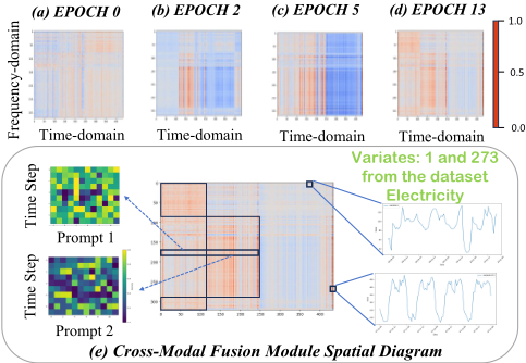
Figure 4 presents a comprehensive case analysis of the CMF module applied to the Electricity dataset for 96-step predictions. The top four subplots, labeled (a) through (d), illustrate the optimization trajectory of the CMF module over different training epochs. The bottom section, represented by subplot (e), provides an in-depth analysis of attention scores during epoch 13.
The left panel specifically explores the correlation between textual prompts and frequency-domain information, highlighting that textual features exhibit a stronger association with frequency-domain characteristics compared to timedomain data. By analyzing specific variables across various time steps and prompts, it becomes apparent that prompts enriched with external information, such as temporal context and dataset segmentation, are particularly effective in revealing latent temporal patterns, including periodicity, under certain conditions.
The right panel explores temporal representations within the time domain. Regions with high attention scores prominently exhibit periodic features, consistent with observations in the frequency domain, whereas regions with low attention scores lack discernible latent patterns. These findings highlight the complementary relationship between textual prompts, frequency-domain features, and temporal representations.
Hyperparameter Sensitivity
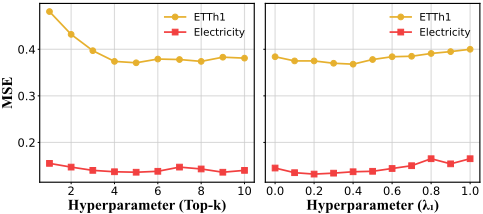
In this section, we investigate the impact of two key parameters in LLM-TPF on the overall performance of the model: 1) The Top-k parameter in the periodic layer of the PFD module, which determines the number of text prototypes introduced and the number of frequency domain layers considered during temporal feature analysis. 2) The regularization loss weight coefficient λ1. In our experiments, we fixed λ2 = 1 in the loss function and set the other two regularization loss weights to be equal for a more comparative analysis.
Figure 5 illustrates the overall performance of the model on the ETTh1 and Electricity datasets with respect to the two key parameters. It can be observed that when the top-k parameter falls within the range of 4 to 6, the model achieves relatively better performance. This is because an appropriate number of textual prototypes facilitates the effective integration of latent temporal features. Conversely, a smaller top-k value may distort critical characteristics of the time series, such as periodicity or trends. The analysis further reveals that a moderate regularization loss weight coefficient λ1 can effectively mitigate the learning bias of large language models. However, an excessively large λ1 can prevent the model from correctly learning sample labels. In summary, hyperparameter design has limited impact, indicating the model's robustness to variations in top-k and λ1.
5 Conclusion
In this paper, we propose LLM-TPF, a model with two personalized branches to capture latent features in time series data, including periodicity. Carefully designed prompts further guide the language model to generate more accurate time series predictions. Furthermore, we incorporate a shared branch to integrate temporal and frequency domain data, enabling LLMs to produce more accurate data representations. Experiments conducted on various datasets demonstrate the accuracy and effectiveness of our model. We hope that future research will further advance the application of LLM-TPF in larger-scale real-world scenarios.
Acknowledgments
This work was supported in part by the National Natural Science Foundation of China under Grants 62476247, 62073295 and 62072409, in part by the "Pioneer" and "Leading Goose" R&D Program of Zhejiang under Grant 2024C01214, and in part by the Zhejiang Provincial Natural Science Foundation under Grant LR21F020003.
@inproceedings{ijcai2025p671,
  title     = {LLM-TPF: Multiscale Temporal Periodicity-Semantic Fusion LLMs for Time Series Forecasting},
  author    = {Pan, Qihong and Tan, Haofei and Shen, Guojiang and Kong, Xiangjie and Wang, Mengmeng and Xu, Chenyang},
  booktitle = {Proceedings of the Thirty-Fourth International Joint Conference on
               Artificial Intelligence, {IJCAI-25}},
  publisher = {International Joint Conferences on Artificial Intelligence Organization},
  editor    = {James Kwok},
  pages     = {6030--6038},
  year      = {2025},
  month     = {8},
  note      = {Main Track},
  doi       = {10.24963/ijcai.2025/671},
  url       = {https://doi.org/10.24963/ijcai.2025/671},
}
TY - CPAPER TI - LLM-TPF: Multiscale Temporal Periodicity-Semantic Fusion LLMs for Time Series Forecasting AU - Pan, Qihong AU - Tan, Haofei AU - Shen, Guojiang AU - Kong, Xiangjie AU - Wang, Mengmeng AU - Xu, Chenyang T2 - Proceedings of the Thirty-Fourth International Joint Conference on Artificial Intelligence, IJCAI-25 PB - International Joint Conferences on Artificial Intelligence Organization PY - 2025 SP - 6030 EP - 6038 DO - 10.24963/ijcai.2025/671 UR - https://doi.org/10.24963/ijcai.2025/671 ER -Copied
Machine-readable versions of this paper, for tools and AI agents:





