
Fast Guaranteed Tensor Recovery with Adaptive Tensor Nuclear Norm
Proceedings of the Thirty-Fourth International Joint Conference on Artificial Intelligence. Main Track. Pages 6057-6065.
https://doi.org/10.24963/ijcai.2025/674
Keywords
- Computer Vision: CV: Machine learning for vision
- Computer Vision: CV: Efficiency and Optimization
- Computer Vision: CV: Low-level Vision
- Machine Learning: ML: Matrix/tensor methods
Abstract
Real-world datasets like multi-spectral images and videos are naturally represented as tensors. However, limitations in data acquisition often lead to corrupted or incomplete tensor data, making tensor recovery a critical challenge. Solving this problem requires exploiting inherent structural patterns, with the low-rank property being particularly vital. An important category of existing low-rank tensor recovery methods relies on the tensor nuclear norms. However, these methods struggle with either computational inefficiency or weak theoretical guarantees for large-scale data. To address these issues, we propose a fast guaranteed tensor recovery framework based on a new tensor nuclear norm. Our approach adaptively extracts a column-orthogonal matrix from the data, reducing a large-scale tensor into a smaller subspace for efficient processing. This dimensionality reduction enhances speed without compromising accuracy. The recovery theories of two typical models are established by introducing an adjusted incoherence condition. Extensive experiments demonstrate the effectiveness of the proposed method, showing improved accuracy and speed over existing approaches. Our code and supplementary material are available at https://github.com/andrew-pengjj/adaptive_tensor_nuclear_norm.
- [Bengua et al., 2017] Johann A Bengua, Ho N Phien, Hoang Duong Tuan, and Minh N Do. Efficient tensor completion for color image and video recovery: Low-rank tensor train. IEEE Transactions on Image Processing, 26(5):2466-2479, 2017.
- [Boyd et al., 2011] Stephen Boyd, Neal Parikh, Eric Chu, Borja Peleato, Jonathan Eckstein, et al. Distributed op- timization and statistical learning via the alternating direc- tion method of multipliers. Foundations and Trends® in Machine learning, 3(1):1-122, 2011.
- [Brbić and Kopriva, 2018] Maria Brbić and Ivica Kopriva. Multi-view low-rank sparse subspace clustering. Pattern recognition, 73:247-258, 2018.
- [Candès et al., 2011] Emmanuel J Candès, Xiaodong Li, Yi Ma, and John Wright. Robust principal component analysis? Journal of the ACM (JACM), 58(3):1-37, 2011.
- [Cichocki et al., 2015] Andrzej Cichocki, Danilo Mandic, Lieven De Lathauwer, Guoxu Zhou, Qibin Zhao, Cesar Caiafa, and Huy Anh Phan. Tensor decompositions for signal processing applications: From two-way to multiway component analysis. 32(2):145-163, 2015.
- [Duan et al., 2016] Yanjie Duan, Yisheng Lv, Yu-Liang Liu, and Fei-Yue Wang. An efficient realization of deep learning for traffic data imputation. Transportation research part C: emerging technologies, 72:168-181, 2016.
- [Faber et al., 2003] Nicolaas Klaas M Faber, Rasmus Bro, and Philip K Hopke. Recent developments in cande- comp/parafac algorithms: a critical review. Chemometrics and Intelligent Laboratory Systems, 65(1):119-137, 2003.
- [Hu et al., 2016] Wenrui Hu, Dacheng Tao, Wensheng Zhang, Yuan Xie, and Yehui Yang. The twist tensor nuclear norm for video completion. IEEE transactions on neural net- works and learning systems, 28(12):2961-2973, 2016.
- [Jiang et al., 2020] Taixiang Jiang, Michael K Ng, Xile Zhao, and Tingzhu Huang. Framelet representation of tensor nu- clear norm for third-order tensor completion. IEEE Trans- actions on Image Processing, 29:7233-7244, 2020.
- [Kilmer et al., 2013] Misha E Kilmer, Karen Braman, Ning Hao, and Randy C Hoover. Third-order tensors as operators on matrices: A theoretical and computational framework with applications in imaging. SIAM Journal on Matrix Analysis and Applications, 34(1):148-172, 2013.
- [Kolda and Bader, 2009] Tamara G Kolda and Brett W Bader. Tensor decompositions and applications. SIAM review, 51(3):455-500, 2009.
- [Kong et al., 2021] Hao Kong, Canyi Lu, and Zhouchen Lin. Tensor q-rank: new data dependent definition of tensor rank. Machine Learning, 110(7):1867-1900, 2021.
- [Liu et al., 2012] Ji Liu, Przemyslaw Musialski, Peter Wonka, and Jieping Ye. Tensor completion for estimating missing values in visual data. IEEE transactions on pattern analysis and machine intelligence, 35(1):208-220, 2012.
- [Liu et al., 2021] Jian Liu, Ce Zhu, Zhen Long, and Yipeng Liu. Tensor regression. Found. Trends Mach. Learn., 14(4):379-565, 2021.
- [Lou and Cheung, 2019] Jian Lou and YiuMing Cheung. Ro- bust low-rank tensor minimization via a new tensor spectral k-support norm. IEEE Transactions on Image Processing, 29:2314-2327, 2019.
- [Lu et al., 2019a] Canyi Lu, Jiashi Feng, Yudong Chen, Wei Liu, Zhouchen Lin, and Shuicheng Yan. Tensor robust principal component analysis with a new tensor nuclear norm. IEEE transactions on pattern analysis and machine intelligence, 42(4):925-938, 2019.
- [Lu et al., 2019b] Canyi Lu, Xi Peng, and Yunchao Wei. Low- rank tensor completion with a new tensor nuclear norm induced by invertible linear transforms. In Proceedings of the IEEE/CVF conference on computer vision and pattern recognition, pages 5996-6004, 2019.
- [Luo et al., 2022] Yisi Luo, Xile Zhao, Taixiang Jiang, Yi Chang, Michael K Ng, and Chao Li. Self-supervised nonlinear transform-based tensor nuclear norm for multi- dimensional image recovery. IEEE Transactions on Image Processing, 31:3793-3808, 2022.
- [McCullagh, 2018] Peter McCullagh. Tensor methods in statistics. Chapman and Hall/CRC, 2018.
- [Ng et al., 2020] Michael K Ng, Xiongjun Zhang, and Xile Zhao. Patched-tube unitary transform for robust tensor completion. Pattern Recognition, 100:107181, 2020.
- [Oseledets, 2011] Ivan V Oseledets. Tensor-train decomposi- tion. SIAM Journal on Scientific Computing, 33(5):2295- 2317, 2011.
- [Peng et al., 2020] Jiangjun Peng, Qi Xie, Qian Zhao, Yao Wang, Leung Yee, and Deyu Meng. Enhanced 3dtv regu- larization and its applications on hsi denoising and com- pressed sensing. IEEE Transactions on Image Processing, 29:7889-7903, 2020.
- [Peng et al., 2022a] Jiangjun Peng, Hailin Wang, Xiangyong Cao, Xinling Liu, Xiangyu Rui, and Deyu Meng. Fast noise removal in hyperspectral images via representative coeffi- cient total variation. IEEE Transactions on Geoscience and Remote Sensing, 60:1-17, 2022.
- [Peng et al., 2022b] Jiangjun Peng, Yao Wang, Hongying Zhang, Jianjun Wang, and Deyu Meng. Exact decom- position of joint low rankness and local smoothness plus sparse matrices. IEEE Transactions on Pattern Analysis and Machine Intelligence, 2022.
- [Peng et al., 2024] Jiangjun Peng, Hailin Wang, Xiangyong Cao, Xixi Jia, Hongying Zhang, and Deyu Meng. Stable local-smooth principal component pursuit. SIAM Journal on Imaging Sciences, 17(2):1182-1205, 2024.
- [Qin et al., 2022] Wenjin Qin, Hailin Wang, Feng Zhang, Jianjun Wang, Xin Luo, and Tingwen Huang. Low-rank high-order tensor completion with applications in visual data. IEEE Transactions on Image Processing, 31:2433- 2448, 2022.
- [Shang et al., 2023] Wenting Shang, Jiangjun Peng, Zebin Wu, Yang Xu, Mohamad Jouni, Mauro Dalla Mura, and Zhihui Wei. Hyperspectral anomaly detection via sparsity of core tensor under gradient domain. IEEE Transactions on Geoscience and Remote Sensing, 2023.
- [Shu et al., 2024] Hao Shu, Hailin Wang, Jiangjun Peng, and Deyu Meng. Low-rank tensor completion with 3-d spa- tiotemporal transform for traffic data imputation. IEEE Transactions on Intelligent Transportation Systems, 2024.
- [Sidiropoulos et al., 2017] Nicholas D Sidiropoulos, Lieven De Lathauwer, Xiao Fu, Kejun Huang, Evangelos E Pa- palexakis, and Christos Faloutsos. Tensor decomposition for signal processing and machine learning. 65(13):3551- 3582, 2017.
- [Signoretto et al., 2014] Marco Signoretto, Quoc Tran Dinh, Lieven De Lathauwer, and Johan AK Suykens. Learning with tensors: a framework based on convex optimization and spectral regularization. Mach. Learn., 94(3):303-351, 2014.
- [Song et al., 2020] Guangjing Song, Michael K Ng, and Xiongjun Zhang. Robust tensor completion using trans- formed tensor singular value decomposition. Numerical Linear Algebra with Applications, 27(3):e2299, 2020.
- [Wang et al., 2012] Naiyan Wang, Tiansheng Yao, Jingdong Wang, and Dit-Yan Yeung. A probabilistic approach to ro- bust matrix factorization. In Computer Vision-ECCV 2012: 12th European Conference on Computer Vision, Florence, Italy, October 7-13, 2012, Proceedings, Part VII 12, pages 126-139. Springer, 2012.
- [Wang et al., 2017] Yao Wang, Jiangjun Peng, Qian Zhao, Yee Leung, Xile Zhao, and Deyu Meng. Hyperspectral im- age restoration via total variation regularized low-rank ten- sor decomposition. IEEE Journal of Selected Topics in Ap- plied Earth Observations and Remote Sensing, 11(4):1227- 1243, 2017.
- [Wang et al., 2021a] Hailin Wang, Feng Zhang, Jianjun Wang, Tingwen Huang, Jianwen Huang, and Xinling Liu. Generalized nonconvex approach for low-tubal-rank ten- sor recovery. IEEE Transactions on Neural Networks and Learning Systems, 33(8):3305-3319, 2021.
- [Wang et al., 2021b] Jianli Wang, Tingzhu Huang, Xile Zhao, Taixiang Jiang, and Michael K Ng. Multi-dimensional visual data completion via low-rank tensor representation under coupled transform. IEEE Transactions on Image Processing, 30:3581-3596, 2021.
- [Wang et al., 2022] Andong Wang, QiBin Zhao, Zhong Jin, Chao Li, and GuoXu Zhou. Robust tensor decomposition via orientation invariant tubal nuclear norms. Science China Technological Sciences, 65(6):1300-1317, 2022.
- [Wang et al., 2023] Hailin Wang, Jiangjun Peng, Wenjin Qin, Jianjun Wang, and Deyu Meng. Guaranteed tensor recovery fused low-rankness and smoothness. IEEE Transactions on Pattern Analysis and Machine Intelligence, 2023.
- [Wu et al., 2022] Tongle Wu, Bin Gao, Jicong Fan, Jize Xue, and Wai Lok Woo. Low-rank tensor completion based on self-adaptive learnable transforms. IEEE Transactions on Neural Networks and Learning Systems, 2022.
- [Xie et al., 2018] Yuan Xie, Dacheng Tao, Wensheng Zhang, Yan Liu, Lei Zhang, and Yanyun Qu. On unifying multi- view self-representations for clustering by tensor multi-rank minimization. International Journal of Computer Vision, 126:1157-1179, 2018.
- [Xu et al., 2019] Wenhao Xu, Xile Zhao, and Michael Ng. A fast algorithm for cosine transform based tensor singular value decomposition. arXiv preprint arXiv:1902.03070, 2019.
- [Yong et al., 2017] Hongwei Yong, Deyu Meng, Wangmeng Zuo, and Lei Zhang. Robust online matrix factorization for dynamic background subtraction. IEEE transactions on pattern analysis and machine intelligence, 40(7):1726- 1740, 2017.
- [Zhang and Aeron, 2016] Zemin Zhang and Shuchin Aeron. Exact tensor completion using t-svd. IEEE Transactions on Signal Processing, 65(6):1511-1526, 2016.
- [Zhang et al., 2019] Hongyan Zhang, Lu Liu, Wei He, and Liangpei Zhang. Hyperspectral image denoising with to- tal variation regularization and nonlocal low-rank tensor decomposition. IEEE Transactions on Geoscience and Remote Sensing, 58(5):3071-3084, 2019.
- [Zhao et al., 2016] Qibin Zhao, Guoxu Zhou, Shengli Xie, Liqing Zhang, and Andrzej Cichocki. Tensor ring decom- position. arXiv preprint arXiv:1606.05535, 2016.
- [Zheng et al., 2012] Yinqiang Zheng, Guangcan Liu, Shigeki Sugimoto, Shuicheng Yan, and Masatoshi Okutomi. Practi- cal low-rank matrix approximation under robust l 1-norm. In 2012 IEEE Conference on Computer Vision and Pattern Recognition, pages 1410-1417. IEEE, 2012.
- [Zhou and Cheung, 2019] Yang Zhou and YiuMing Cheung. Bayesian low-tubal-rank robust tensor factorization with multi-rank determination. IEEE Transactions on Pattern Analysis and Machine Intelligence, 43(1):62-76, 2019.
- [Zhou and Tao, 2011] Tianyi Zhou and Dacheng Tao. Godec: Randomized low-rank & sparse matrix decomposition in noisy case. In Proceedings of the 28th International Con- ference on Machine Learning, ICML 2011, 2011.
- [Zhou et al., 2012] Xiaowei Zhou, Can Yang, and Weichuan Yu. Moving object detection by detecting contiguous out- liers in the low-rank representation. IEEE transactions on pattern analysis and machine intelligence, 35(3):597-610, 2012.
References were extracted automatically from the PDF and may contain errors.
Full text extracted automatically from the PDF; figures, tables and equations may differ. The PDF is the version of record.
1 Introduction
Tensors (or multidimensional arrays) naturally represent diverse real-world data, such as multi-spectral images [Wang et al., 2017; Peng et al., 2020], multi-view task[Brbi´c and Kopriva, 2018; Xie et al., 2018], and intelligence system data [Shu et al., 2024; Duan et al., 2016]. Their ability to preserve multidimensional structure with accuracy has made tensor analysis a key focus in fields like statistics [McCullagh, 2018], signal processing [Cichocki et al., 2015; Sidiropoulos et al., 2017], machine learning [Signoretto et al., 2014; Liu et al., 2021], and computer vision [Bengua et al., 2017; Zhang et al., 2019; Hu et al., 2016]. However, due to limitations in acquisition equipment and complex environments, tensor data often contain noise and missing values [Peng et al., 2024], which compromise the accuracy of subsequent tasks such as detection and recognition [Shang et al., 2023]. Fortunately, tensor data inherently contains abundant priors, and leveraging these can help achieve higher-quality tensor data.
∗Corresponding author
Among the various priors for tensor data, low-rankness is one of the most crucial[Kolda and Bader, 2009]. This prior assumes that the tensor resides within a low-dimensional subspace, enabling the capture of its global correlations. Numerous studies have demonstrated that most real-world tensors exhibit low-rank structures, which leads to the following lowrank tensor recovery model,
where R(·) denotes certain tensor low-rankness regularizer, Φ(·) models the tensor degradation, e.g., data missing or noise corruption, corresponding to tensor completion (TC) and tensor robust principal component analysis (TRPCA).
Different from the rank of a matrix, there are various notions of tensor rank with different tensor decompositions. The classical ones contain CANDECOMP/PARAFAC (CP) [Faber et al., 2003], Tucker [Wang et al., 2017] and Sum Nuclear Norm (SNN) [Liu et al., 2012]. In the last few years, several new low-rank tensor approximation frameworks have been proposed, such as tensor train [Oseledets, 2011], tensor ring [Zhao et al., 2016], and tensor singular value decomposition (t-SVD) [Kilmer et al., 2013]. While many tensor decomposition methods exist, most, except for the tensor nuclear norm (TNN) [Lu et al., 2019a; Qin et al., 2022], based on t-SVD, lack a solid tensor recoverable theory[Zhang and Aeron, 2016]. In addition, since tensor decomposition involves more complex algebraic operations than matrices and the large size of tensor data, the efficiency of tensor decomposition is often relatively low [Kolda and Bader, 2009].
Since the tensor nuclear norm has good theoretical properties, its variants have attracted widespread attention. The tensor nuclear norm focuses on how to characterize the low rank of data in the transformation domain [Kilmer et al., 2013]. For a third-order tensor T ∈ Rn1×n2×n3 , assuming that its third mode has a low-rank property, the transformed tensor T ∈ Rn1×n2×n3 can be obtained as follows:
| Methods | TNN | DCTNN | UTNN | WTNN | CTNN | FTNN | S2NTNN | Q-rank | ATNN |
|---|---|---|---|---|---|---|---|---|---|
| Transform | FFT | DCT | Unitary | Wavelet | Couple | Framelet | DNN | Unitary | COM |
| Learnable? | � | � | � | � | � | � | � | � | � |
| Theory? | � | � | � | � | � | � | � | � | � |
| Time Complexity | O(n21 n2n3) | O(n21 n2n3) | O(n21 n2n3) | O(n21 n2n3) | O(n21 n2n3) | O(n21 n2n3) | O(n21 n2n3) | O(n21 n2n3) | O(n21 n2r3) |
where ×3 denotes mode-3 tensor product [Kolda and Bader, 2009], and L ∈ Rn3×n3 is the corresponding transformed matrix. The tensor tubal rank is defined as the summation of the matrix ranks of all slices of the transformed domain tensor T . To encode the low-rank property, the tensor nuclear norm is introduced, which is computed as the summation of the nuclear norms of each slice of T . Mathematically, it is expressed as:
Initially, the transformed matrix L was fixed as the discrete Fourier matrix (DFT) [Kilmer et al., 2013; Zhang and Aeron, 2016]. Later, it was found that defining different transformed matrices could enhance the low-rank property in certain cases within the transform domain [Lu et al., 2019a]. As a result, a series of works have emerged focused on the choice of transformed matrices, such as TNN based on the discrete cosine transform (i.e., DCTNN ) [Xu et al., 2019; Lu et al., 2019b], the wavelet transform (i.e., WTNN) [Ng et al., 2020], the unitary matrix (i.e., UTNN) [Song et al., 2020], the Couple transform (i.e., CTNN) [Wang et al., 2021b], the Framelet transform (i.e., FTNN) [Jiang et al., 2020], the data-independent transform (i.e., Q-rank) [Kong et al., 2021], the neural network (i.e., S2NTNN) [Luo et al., 2022] and many others [Zhou and Cheung, 2019; Lou and Cheung, 2019; Wang et al., 2021a; Wu et al., 2022]. Although these TNN variants have achieved promising results in specific cases, they face several common challenges:
- Nonlinear transformation-based models lack the theoretical guarantee of exact recovery inherent to TNN;
- Most models assume the transformation matrix is full rank, limiting their ability to significantly enhance the tensor's low-rank property in the transformed domain;
- Full-rank transformation matrices can not reduce the data size of tensors in the transformed domain, leading to low computational efficiency.
To address the aforementioned limitations, this paper proposes a new TNN scheme with both computational validity and theoretical guarantee. Specifically, we propose to adaptively learn a column-orthogonal transformation matrix (COM) from the data, and the proposed TNN is then induced under such COM transform. We refer it as Adaptive Tensor Nuclear Norm (ATNN). Equipped with the ATNN, we strictly prove the exact recovery theories for two typical tensor recovery models, TC and TRPCA. For easy comparison, we summarize the key characteristics of several existing TNN variants in Table 1, from which we can find that that only the ATNN model stands out by effectively balancing data adaptability, theoretical guarantees, and computational efficiency, particularly when the third-mode rank r3 is much smaller than n3 for a third-order tensor T ∈ Rn1×n2×n3 . In summary, this paper makes four key contributions:
Data-Adaptive Transformation: The transformation matrix in ATNN is adaptively learned from the data, allowing it to adapt to different datasets. This adaptability provides a significant advantage over the existing fixed transformation matrices.
High Computational Efficiency: The learned columnorthogonal transformation matrix can reduce the size of the tensor in the transformed domain, especially for data with strong low-rank properties in the third mode. This leads to high computational efficiency. Unlike all existing TNN variants using full-rank transformation matrices, column-orthogonal matrices explicitly model the low rank of the tensor's third modality, offering superior representation of the tensor's lowrank structure.
Exact Recovery Theory: It is proved that when the transformation matrix is not full rank, the ATNN-based TC and TRPCA problem can still be guaranteed with exact recovery, provided that the number of columns in the transformation matrix exceeds the third-mode rank of the tensor.
Superior Balanced Performance: Extensive numerical and real-world experiments demonstrate that the ATNN framework achieves superior balanced performance between recovery accuracy and time cost across nearly all datasets and tasks compared with many state-of-the-art methods.
The organization of this paper is as follows: the notation, definition, and analysis are given in Section 2. The ATNN definition and its derived models are given in Section 3. The theoretical results are given in Section 4. The simulated and real experiments are conducted in Sections 5. The conclusion is given in Section 6.
2 Notations and Preliminaries
We first introduce the high-order t-SVD framework briefly. For an order-d tensor T ∈ Rn1×n2×···×nd , T (i1, i2, · · · , id) denotes its (i1, i2, · · · , id)-th element, T (:, :, i3, · · · , id) denotes its (i3, · · · , id)-th frontal slice, and Ti := T (:, · · · , : , i) denotes its i-th order-(d - 1) component. Slice T (: , :, i3, · · · , id) is also written as Tj with index j = i3 + (i4 - 1)n3 + · · · + (id - 1)n3 · · · nd-1. unfold(T ) := [T1, T2, · · · , Tnd ]T ∈ Rn1nd×n2×···×nd-1 is the unfold operator and fold(·) is its inverse operator satisfying fold(unfold(T )) = T . bunfold(T ) ∈ Rn1n3···nd×n2 is the matrix formed by using unfold(·) repeatedly. Denote
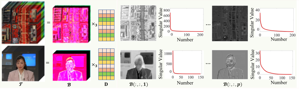
(a) Low-rank Decomposition among three-mode
(b) Low-rank Properties of Each Slice of Transformed Domain 𝓑
Figure 1: Demonstration of the idea of data adaptive transformed matrix construction and low rank property of transformed domain.
as T 's circulant unfolding sized n1nd ×· · ·×nd-2nd ×nd-1, bcirc(T ) as its block circulant matrix at the base level of circ(T ) sized n1n3 · · · nd × n2n3 · · · nd, and block diagonal matrix bdiag(T ) = diag(T1 ,T2 , · · · ,TJ ), where J = n3 · · · nd. bdiag(T ) is also written as T for brevity.
The t-SVD framework [Qin et al., 2022] takes high-order tensor-tensor product with invertible linear transform as its cornerstone. For an invertible linear transform L, TL := L(T ) = T ×3 Un3 ×4 · · · ×d Und , where ×i denotes mode-i product and Uni is transform matrix sized ni × ni, such as the Discrete Fourier Transform (DFT) and Discrete Cosine Transform (DCT) matrices. Its inverse L-1 (T ) = T ×3 U-1 n3 ×4 · · · ×d U-1 nd and L-1 (L(T )) = T . Note {Uni }di=1 are assumed satisfying (U∗nd ⊗U∗nd-1 ⊗ · · · ⊗U∗n3 ) · (Und ⊗ Und-1 ⊗ · · · ⊗ Un3 ) = ℓ · In3···nd , where ⊗ is Kronecker product and ℓ > 0 is only a transform specific scale constant, e.g., F∗nFn = n · In for n × n DFT matrix Fn and C∗nCn = 1 · In for n × n DCT matrix Cn.
Definition 1 (order-d tensor-tensor product). For order-d tensors A ∈ Rn1×l×···×nd and B ∈ Rl×n2×···×nd , its transform L based product is defined as
where ∆ denotes face-slice-wise product (C = A∆B ⇔ Cj = Aj · Bj , ∀j = 1, · · · , n3 · · · nd).
By using the following property that the transform L can diagonalize the block circulant matrix bcirc(T ) using the following property (ˆU ⊗ In1 ) · bcirc(T ) · (ˆU-1 ⊗ In2 ) = bdiag(TL) := TL, where ˆU := Und ⊗Und-1 ⊗ · · · ⊗Un3 , ˆU-1 := U-1 nd ⊗U-1 nd-1 ⊗ · · · ⊗ U-1 n3 . Further, it derives that C = A ∗L B is equivalent to CL = AL · BL, which leads a simple implement for (4) via matrix-matrix multiplication.
Definition 2 (transpose tensor). For T ∈ Rn1×n2×···×nd , its transpose T T ∈ Rn2×n1×···×nd satisfies that T T L (:, : , i3, · · · , id) = TL(:, :, i3, · · · , id)T for all ij = 1, · · · , nj.
Definition 3 (identity tensor). An order-d tensor I ∈ Rn×n×···×nd is called identity tensor if it satisfies that IL(:, : , i3, · · · , id) = In for all ij = 1, · · · , nj.
Definition 4 (orthogonal tensor). An order-d tensor U ∈ Rn×n×···×nd is called orthogonal tensor if it satisfies that U T ∗L U = U ∗L U T = In.
Definition 5 (f-diagonal tensor). An order-d tensor T ∈ Rn×n×···×nd is called f-diagonal tensor if it satisfies that T (:, :, i3, · · · , id) is diagonal for all ij = 1, · · · , nj.
Theorem 1 (order-d t-SVD). For any order-d tensor T ∈ Rn1×n2×···×nd , it can be decomposed as
where U ∈ Rn1×n1×···×nd and V ∈ Rn2×n2×···×nd are orthogonal, and S ∈ Rn1×n2×···×nd is an f-diagonal tensor.
Same as the normal t-SVD with DFT transform [Kilmer et al., 2013], the above arbitrary invertible linear transforms induced t-SVD can be realized by performing SVD on each slice of TL in transformed domain and then inverting the corresponding components back to original domain. Moreover, the following relationship has been verified by using inverse transform, S(i, i, 1, · · · , 1) = 1ℓ ∑n3 i3=1 · · · ∑nd id=1 SL(i, i, i3, · · · , id), which leads the nonincreasing property of S(i, i, 1, · · · , 1). Thus it is often called tensor singular values. Similarly, the t-SVD has a skinny form [Qin et al., 2022] with the following t-SVD rank, and further some concepts can be established.
Definition 6 (order-d t-SVD rank & TNN). For order-d tensor T ∈ Rn1×n2×···×nd with t-SVD T = U ∗LS ∗LV T, its t-SVD rank is defined as
where ♯ denotes the cardinality of a set. Its tensor nuclear norm (TNN) is defined as
3 Tensor Recovery via Adaptive Tensor Nuclear Norm Minimization
Next, we explain the reasons for constructing the Adaptive Tensor Nuclear Norm (ATNN) and how to construct the ATNN.
3.1 ModelingMotivation
Considering that many tensor data types (such as hyperspectral data and video data shown in Figure 1 inherently exhibit low-rank properties across third-mode, performing a lowrank tensor decomposition can transform a large-scale tensor T ∈ Rn1×n2×n3 into the product of a smaller-scale tensor B ∈ Rn1×n2×r3 , (r3 ≤ n3) and a matrix D ∈ Rn3×r3 . It is widely recognized that defining regularization on this smallerscale tensor can lead to efficient solution models [Peng et al., 2022a]. As shown in Figure 1, each slice of B has a low-rank property. Characterizing the low-rank properties of slices of transform domain data is exactly the original intention of the tensor nuclear norm.
Therefore, combining the findings in Figure 1 and the original intention of the tensor nuclear norm, we thought of defining the nuclear norm on the smaller-scale tensor B. Under this definition, D obtained by low-rank decomposition from each data acts as a transformed matrix and this transformed matrix is data adaptive.
3.2 Data Adaptive Transformation
Next, we define data-adaptive transformation. For a thirdorder tensor T ∈ Rn1×n2×n3 , assuming that its third mode has low-rank property with rank r3, it can be factorized as
where ×3 denotes mode-3 tensor product, B ∈ Rn1×n2×r3 , D ∈ Rn3×r3 satisfying DT D = I and r3 = Rank(T(3)). According to low-rank tensor decomposition (8), we have
Therefore, if we regard B as a transformed tensor TL = L(T ) = T = T ×3DT in Eq. (2), the column-orthogonal matrix (COM) DT can be regarded as the transform matrix, and D is the inverse transform of DT . Theorem 2 demonstrates that the matrix D, which validates the equation T = B ×3 D, is appropriately suited to act as a transformed matrix.
Theorem 2. For a three-order tensor T = B ×3 D ∈ Rn1×n2×n3 composed of B ∈ Rn1×n2×r3 and D ∈ Rn3×r3 , if the transformation matrix is chosen as DT , the information of the data before and after the transformation will not be lost.
3.3 Adaptive Tensor Nuclear Norm
After defining the data-adaptive transformation, the ATNN of T can be reformulated as:
Eq. (10) limits the column orthogonality of the transformation for two purposes. One is the need to keep the information in the transformed domain from being lost in Theorem 2, and the other is that as Theorem 3 below shows, the column orthogonal transformation can effectively reduce the objective value of the ATNN model (10).
Theorem 3. For the ATNN model (10), we have the following two assertions:
a) The upper bound objective of the ∥T ∥⊛,A is ∥T(3)D∥2,1. b) If the transformed matrix is set as the component matrix of tensor T , then the upper bound objective can obtain the smallest value.
3.4 Tensor RecoveryModels Based on ATNN
Next, we consider two common types of recovery tasks, tensor robust principal component analysis (TRPCA) and tensor completion (TC) tasks.
The observed tensor and the tensor needed to be recovered are denoted as Y and T0, respectively. For TC tasks, the observation Y has the support set Ω ∼ Ber(ρ), i.e., PΩ(Y) = PΩ(T0). For TRPCA tasks, the observation Y is corrupted with a sparse component E0 (which may represent foreground or sparse noise), denoted as Y = T0 + E0. Combining ATNN with TC and TRPCA tasks, we can obtain the following ATNNTCmodel (11) and ATNN-RPCAmodel (12).
and
3.5 Optimization
This part derives efficient algorithms for solving the ATNNRPCA (12) and ATNN-TC (11) using the ADMM framework [Boyd et al., 2011]. We first write the augmented Lagrangian function of the ATNN-TC program as
and that of the ATNN-RPCA program as:
where µ is the penalty parameter and Λ is the lagrange multiplier. The idea of the ADMM algorithm is to alternately update each variable. For Eq. (13), we need to solve the following three subproblems in Eq. (15).
The optimization problem (12) also involves solving four sub-problems. Based on Eq. (15), we only need to replaced the subproblem about E with E := minE λ∥E∥1+ µ2 ∥Y-B×3 D - E + Λ/µ∥2F to complete the entire optimization process for Eq. (12). Due to page limitations, the update procedures, detailed optimization steps and convergence guarantees are provided in the supplementary material.
3.6 Efficiency Analysis of ATNN
Although the previous section did not detail the algorithms for ATNN, we can still compare the time complexity of TNNbased TRPCA and TC models, as their update steps follow the same procedure as Eq. (15). Among the four subproblems, updating the transformed variable B is the most timeconsuming. For a tensor T ∈ Rn1×n2×n3 , if the transform matrix D ∈ Rn3×n3 is full-rank, the soft-thresholding step has complexity O(n21n2n3). In contrast, with a compact orthogonal matrix D ∈ Rn3×r3 under our ATNN framework, the transformed data size becomes n1 × n2 × r3, reducing the complexity to O(n21n2r3). When r3 ≪ n3, this leads to a significant efficiency gain, as confirmed in our experiments.
4 Theoretical Guarantees
With ATNN defined above, we now consider the exact recovery guarantee of ATNN-RPCA in (12) and ATNN-TC in (11). The problem of TRPCA is to recover a low tubal rank tensor T0 from highly corrupted measurements Y = T0 + E. The problem of TC is to recover a low tubal rank tensor T0 from the partly observed measurements Y = PΩ(T0). In this section, we show that under certain assumptions, the low tubal rank tensor T0 can be exactly recovered by solving program (11), and the low tubal rank tensor T0 and sparse part E0 can be exactly recovered by solving program (12).
4.1 Tensor Incoherence Condition
Among all the assumptions, the incoherence condition [Candès et al., 2011; Lu et al., 2019a; Wang et al., 2023] is the most important one, which stipulates that the element distribution of the orthogonal left and right singular value tensors obtained under t-SVD decomposition is as dispersed as possible. Next, we define the incoherence condition based on the COM D extracted from the data when used as the transformed operator. Similar to the tensor incoherence conditions defined in [Lu et al., 2019a], the tensor incoherence conditions based on the COM D are defined as follows:
Definition 7 (Tensor Incoherence Conditions). For T0 ∈ Rn1×n2×n3 with t-SVD rank R, it has the skinny t-SVD T0 = U ∗D S ∗D V T . Then T0 is said to satisfy the tensor incoherence conditions with parameter µ if
where˚ei,˚ej are the tensor column basis defined in [Lu et al., 2019a].
It is worth noting that in previous incoherence conditions [Lu et al., 2019a], the transformations were all full-rank matrices, whereas we are the first to propose a definition based on non-full-rank matrices. In addition, since the upper limit of ∥U T ∗D˚ei∥F is R, it can be deduced that the upper limit of µ is O(n1), which is much smaller than O(n1n3) in previous works [Lu et al., 2019a; Wang et al., 2023]. From Eqs. (17) and (18), it can be seen that the sample size is proportional to µ, while the tensor's tubal rank is inversely proportional to µ. Thus, a smaller µ relaxes the theorem's conditions and broadens the model's applicability.
4.2 Main Results
Next, we now demonstrate that both the model (11) and (12) possess exact recovery capability, and the proof of the following two theorems are placed in supplemental materials.
Theorem 4 (TC Theorem). Suppose that T0 ∈ Rn×n×n3 in the ATNN-TC model (11) obeys the tensor incoherence conditions (16) and the support set Ω ∼ Ber(p). Then, there exist universal constants c0, c1, c2 > 0 such that T0 is the unique solution to model (11) with probability at least 1 - c1(nn3)-c2 , i.e., ˆ T = T0, provided that
Theorem 5 (TRPCA Theorem). Suppose that T0 ∈ Rn×n×n3 in ATNN-RPCA model (12) obeys the tensor incoherence conditions (16) and E0's support set, denoted as Ω0, is uniformly distributed among all sets of cardinality m. Then, there exist universal constants c1, c2 > 0 such that (T0, E0) is the unique solution to model (12) when λ = 1/√n with probability at least 1- c1(nn3)-c2 , i.e., ( ˆ T , ˆ E) = (T0, E0), provided that
rankt(T0) ≤ ρrµ-1n log-2 (n) and m≤ ρsn2n3, (18) where ρr, ρs > 0 are some numerical constants.
5 Experiments
Next, we conducted numerical experiments to validate Theorems 4 and 5. Based on Theorem 5, λ was set to 1/√max{n1, n2} for all TRPCA tasks. While this theoretical value serves as a practical guideline, performance can be further improved by fine-tuning λ. All simulations were performed on a PC with an Intel Core i5-10600KF 4.10 GHz CPU, 32 GB RAM, and a GeForce RTX 3080 GPU (10 GB).
5.1 Simulated Experiments
We generate a tensor with tubal rank R as a product T0 = P ∗L QT , where P and Q are n × R × n tensors with entries independently sampled from N(0, 1/n) distribution and the COM L ∈ Rr3×n is generated by orthogonalizing the random matrix with entries independently sampled from N(0, 1). For the TRPCA task, the support set Ω (with size m) of E0 with independent Bernoulli ±1 entries is chosen uniformly at random, and the observation tensor is set as: Y = T0 + E0. For the TC tasks, the observation Y is set as Y = PΩ(T0).
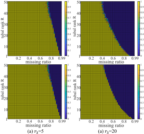
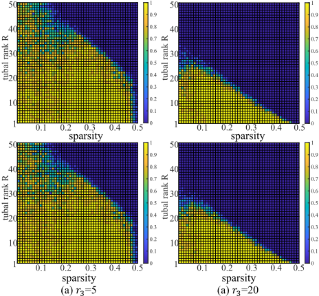
Next, we investigate how the tubal rank of T0 and the sparsity of E0 (and missing ratio of T0 ) affect the performance of model (11) and (12). We consider n = 50 and two values of r3, i.e., r3 = 5, 20. We vary the sparsity ρsof E0 as [0.01 : 0.01 : 0.5], the missing ratio ρ of T0 as [0.01 : 0.02 : 0.99], and tubal rank of T0 as [1 : 1 : 50], respectively. For each combination of (R, ρs) and (R, ρ), we perform 10 test instances and declare a trial successful if the relative recovered error is less than 0.01. The fraction of successful recoveries are plotted in Figures 2 and 3. Here, we set up two modes: in the first row of Figures 2 and 3, the transformed matrix is adaptively learned from the data, while in the second row, the optimal transformed matrix is predefined. From Figures 2 and 3, we observe that there is a significant region where the recovery is correct for both models. Furthermore, two notable phenomena can be observed: 1) The phase transition diagram in the first row of Figures 2 and 3 closely resembles the second row, indicating that even if we don't know the correct COM L in the models (11) and (12), we can also learn the COM L; 2) The phase transition diagram of r3 = 5 is much better than that of r3 = 20 for both TRPCA and TC tasks, which shows that it is necessary to consider the low-rank property of mode 3.
| Methods | WDC | PaviaU | Beans | Cloth | ||||
|---|---|---|---|---|---|---|---|---|
| PSNR | Times | PSNR | Times | PSNR | Times | PSNR | Times | |
| LRMC | 18.53 | 24.38 | 15.17 | 2.93 | 15.96 | 7.61 | 13.11 | 10.95 |
| HaLRTC | 22.09 | 54.37 | 18.87 | 30.34 | 20.62 | 64.48 | 19.01 | 92.65 |
| RPCA | 32.08 | 28.99 | 24.98 | 6.59 | 17.88 | 17.92 | 18.47 | 18.28 |
| SNN | 26.02 | 136.2 | 31.34 | 121.1 | 16.14 | 176.2 | 16.77 | 176.7 |
| KBR | 22.64 | 167.2 | 20.91 | 58.63 | 20.26 | 252.1 | 20.91 | 162.9 |
| TNN | 19.62 | 419.2 | 17.09 | 120.2 | 20.39 | 322.4 | 15.51 | 324.8 |
| CTNN | 17.21 | 485.7 | 15.38 | 130.7 | 15.64 | 363.4 | 14.55 | 353.9 |
| CTV | 33.85 | 170.2 | 31.91 | 41.85 | 29.35 | 103.8 | 27.33 | 102.2 |
| TCTV | 32.12 | 815.2 | 29.62 | 172.5 | 32.85 | 641.3 | 27.36 | 627.9 |
| Ours | 39.82 | 21.34 | 35.31 | 5.32 | 29.46 | 29.22 | 27.53 | 19.30 |
| Methods | data | Times | ||||||
|---|---|---|---|---|---|---|---|---|
| airp. | shop. | lobb. | esca. | curt. | foun. | Aver. | ||
| RPCA | 0.872 | 0.945 | 0.913 | 0.905 | 0.872 | 0.942 | 0.899 | 2.37 |
| GODEC | 0.900 | 0.919 | 0.856 | 0.913 | 0.913 | 0.910 | 0.902 | 0.64 |
| DECOLOR | 0.863 | 0.946 | 0.924 | 0.908 | 0.886 | 0.944 | 0.895 | 8.29 |
| OMoGMF | 0.914 | 0.948 | 0.925 | 0.911 | 0.905 | 0.942 | 0.917 | 3.92 |
| RegL1 | 0.898 | 0.942 | 0.882 | 0.416 | 0.890 | 0.919 | 0.850 | 10.74 |
| PRMF | 0.891 | 0.942 | 0.882 | 0.907 | 0.881 | 0.917 | 0.901 | 13.68 |
| CTV | 0.918 | 0.954 | 0.934 | 0.915 | 0.871 | 0.938 | 0.918 | 10.28 |
| TNN | 0.522 | 0.661 | 0.631 | 0.598 | 0.582 | 0.578 | 0.595 | 16.87 |
| CTNN | 0.686 | 0.684 | 0.661 | 0.658 | 0.699 | 0.545 | 0.630 | 17.39 |
| ATNN | 0.919 | 0.948 | 0.936 | 0.916 | 0.916 | 0.946 | 0.923 | 2.32 |
| Methods | WDC | PaviaU | Beans | Cloth | ||||
|---|---|---|---|---|---|---|---|---|
| PSNR | Times | PSNR | Times | PSNR | Times | PSNR | Times | |
| LRMC | 18.53 | 24.38 | 15.17 | 2.93 | 15.96 | 7.61 | 13.11 | 10.95 |
| HaLRTC | 22.09 | 54.37 | 18.87 | 30.34 | 20.62 | 64.48 | 19.01 | 92.65 |
| KBR | 31.42 | 1589 | 29.92 | 725.7 | 26.06 | 1253 | 24.14 | 1292 |
| TNN | 30.01 | 1019 | 26.43 | 207.9 | 26.10 | 419.2 | 23.46 | 441.2 |
| CTNN | 33.36 | 378.9 | 31.69 | 114.4 | 27.61 | 129.6 | 25.71 | 136.2 |
| UTNN | 27.89 | 487.6 | 21.80 | 156.3 | 17.28 | 116.6 | 16.27 | 117.9 |
| FTNN | 34.87 | 4376 | 32.56 | 1263 | 28.48 | 1587 | 25.25 | 2054 |
| OITNN | 32.92 | 838.2 | 28.46 | 292.4 | 27.28 | 448.6 | 24.06 | 391.8 |
| TCTV | 33.33 | 2116 | 31.81 | 861.4 | 31.77 | 1570 | 28.38 | 1488 |
| S2NTNN | 37.36 | 168.7 | 35.15 | 40.78 | 27.44 | 104.2 | 31.28 | 113.2 |
| Ours | 38.06 | 232.4 | 33.94 | 58.34 | 28.83 | 156.3 | 25.81 | 142.4 |
5.2 Real Experiments
To validate the effectiveness of the proposed ATNN models for tensor recovery, we conducted experiments on various datasets, including hyperspectral images (HSI), multispectral images (MSI), color video images, and surveillance videos. Due to space constraints, detailed results on robustness analysis, parameter settings, and convergence verification are provided in the supplementary material.
For a comprehensive comparison, we included additional state-of-the-art methods not listed in Table 1. These include CTV [Peng et al., 2022b] and TCTV [Wang et al., 2023] for the TRPCA task, LRMC [Candès et al., 2011], HaLRTC [Liu et al., 2012], UTNN [Ng et al., 2020], and OITNN [Wang et al., 2022] for the TC task, as well as GODEC [Zhou and Tao, 2011], DECOLOR [Zhou et al., 2012], OMoGMF [Yong et al., 2017], RegL1 [Zheng et al., 2012], and PRMF [Wang et al., 2012] for background modeling. Prior to the experiments, the gray values of each band were normalized to the [0, 1] range using the max-min formula.
| Methods | Akiyo | Foreman | Carphone | News | ||||
|---|---|---|---|---|---|---|---|---|
| PSNR | Times | PSNR | Times | PSNR | Times | PSNR | Times | |
| LRMC | 10.81 | 8.06 | 8.79 | 7.21 | 11.57 | 6.92 | 13.27 | 13.41 |
| HaLRTC | 17.66 | 61.04 | 15.55 | 44.87 | 14.20 | 42.46 | 16.43 | 87.63 |
| KBR | 29.76 | 689.2 | 23.97 | 668.2 | 26.49 | 798.2 | 26.42 | 1043 |
| TNN | 31.94 | 217.5 | 23.15 | 181.5 | 26.27 | 493.6 | 28.56 | 249.6 |
| CTNN | 28.63 | 192.0 | 22.13 | 152.7 | 25.06 | 196.2 | 25.59 | 174.7 |
| UTNN | 21.72 | 172.4 | 16.51 | 167.6 | 20.24 | 202.7 | 21.21 | 162.6 |
| FTNN | 30.74 | 1258 | 22.97 | 1123 | 25.43 | 1335 | 28.77 | 1494 |
| OITNN | 32.68 | 397.5 | 23.89 | 296.7 | 27.14 | 472.3 | 29.43 | 322.3 |
| TCTV | 33.41 | 874.8 | 26.69 | 821.4 | 29.10 | 1103 | 30.65 | 772.2 |
| S2NTNN | 33.16 | 168.7 | 23.57 | 83.98 | 27.33 | 100.7 | 29.11 | 90.61 |
| Ours | 33.74 | 95.89 | 24.16 | 78.21 | 27.44 | 80.11 | 29.72 | 78.94 |
Tensor Robust Principal Component Analysis Task
In this part, we conducted experiments using three types of data across two tasks: HSI, MSI, and video surveillance data. The HSI tasks include the paviaU and WDC datasets, while the MSI consists of the Beans and Cloth datasets from the CAVE collection. The video surveillance data is sourced from the Li dataset, with detailed information available in the supplementary material.
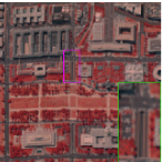
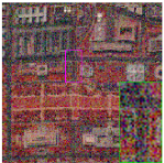
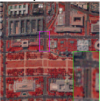
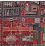
The two tasks we focused on were sparse noise denoising and foreground-background separation. For sparse noise denoising, salt-and-pepper noise was added at levels ranging from 0.1 to 0.6. Table 1 presents the denoising performance of all methods under a salt-and-pepper noise variance of 0.6, while Table 2 shows the AUC values for the video surveillance task. As observed in Tables 2 and 3, the proposed ATNN method outperforms not only other TNN variants but also models that combine low-rank and local smoothness, achieving superior performance with lower computational time. Furthermore, in Figure 4, we provide recovery results from various methods. The figure clearly demonstrates that ATNN restores better details compared to the other methods. These results validate the effectiveness and robustness of the proposed method and its underlying theoretical foundation.
Tensor Completion Task
In this part, we conducted tensor completion experiments on three types of data: HSI data, MSI and color video data. The newly added color video data includes four datasets: Akiyo, Foreman, Carphone, and News. Test samples were generated by introducing random missing values, with the missing rate ranging from 80% to 99%. Tables 4 and 5 present the experimental results of all the competing methods under a missing rate higher than 95%. From the tables, it is evident that ATNN

ATNN: 37.47/0.985
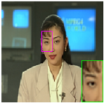
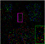
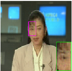
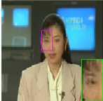
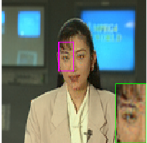
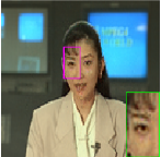
Figure 5: Recovered images of all competing methods under sample ratio of 0.05 on the 10th frame of Akiyo data.
outperforms all TNN variant models and consistently ranks the top one. Furthermore, the image restoration results are shown in Figure 5.
6 Conclusion
In this paper, we introduce an efficient and self-adaptive learnable transformed tensor nuclear norm framework with provable recovery guarantees. Specifically, our approach leverages the low-rank property of the third mode of the tensor to represent the tensor to be repaired as a combination of a smallsized tensor and a column-orthogonal matrix. The columnorthogonal matrix serves as an adaptively learned transform matrix derived from the data. By employing the nuclear norm on the small-sized tensor, our ATNN model can obtain higher computational efficiency compared to existing methods. Additionally, we established the exact recoverable theorem for the ATNN model with a column-orthogonal transform matrix. Extensive experimental results demonstrate the effectiveness of our approach and the validity of our theoretical findings.
Acknowledgments
This work was in part by the National Natural Science Foundation of China under Grant 12401674, 62272375, 12201497 and 124B2029, the Guangdong Basic and Applied Basic Research Foundation under Grant 2025A1515011453, the Fundamental Research Funds for the Central Universities under Grant D5000240095, and the Key Research, Development Plan of Shaanxi Province, China (No. 2024GX-YBXM-145).
@inproceedings{ijcai2025p674,
  title     = {Fast Guaranteed Tensor Recovery with Adaptive Tensor Nuclear Norm},
  author    = {Peng, Jiangjun and Wang, Hailin and Cao, Xiangyong and Xu, Shuang},
  booktitle = {Proceedings of the Thirty-Fourth International Joint Conference on
               Artificial Intelligence, {IJCAI-25}},
  publisher = {International Joint Conferences on Artificial Intelligence Organization},
  editor    = {James Kwok},
  pages     = {6057--6065},
  year      = {2025},
  month     = {8},
  note      = {Main Track},
  doi       = {10.24963/ijcai.2025/674},
  url       = {https://doi.org/10.24963/ijcai.2025/674},
}
TY - CPAPER TI - Fast Guaranteed Tensor Recovery with Adaptive Tensor Nuclear Norm AU - Peng, Jiangjun AU - Wang, Hailin AU - Cao, Xiangyong AU - Xu, Shuang T2 - Proceedings of the Thirty-Fourth International Joint Conference on Artificial Intelligence, IJCAI-25 PB - International Joint Conferences on Artificial Intelligence Organization PY - 2025 SP - 6057 EP - 6065 DO - 10.24963/ijcai.2025/674 UR - https://doi.org/10.24963/ijcai.2025/674 ER -Copied
Machine-readable versions of this paper, for tools and AI agents:





