
QuantileFormer: Probabilistic Time Series Forecasting with a Pattern-Mixture Decomposed VAE Transformer
Proceedings of the Thirty-Fourth International Joint Conference on Artificial Intelligence. Main Track. Pages 6147-6155.
https://doi.org/10.24963/ijcai.2025/684
Keywords
- Data Mining: DM: Mining spatial and/or temporal data
- Machine Learning: ML: Time series and data streams
Abstract
Probabilistic time series forecasting has attracted an increasing attention in machine learning community for its potential applications in the fields of renewable energy, traffic management, healthcare, etc. Previous research mainly focused on extracting long-range dependencies for point-wise prediction, which fail to capture complex temporal patterns and statistical characteristics for probabilistic analysis. In this paper, we propose a novel pattern-mixture decomposition method that decomposes long-term series into quantile drift, divergence patterns, and Gaussian mixture components, which can effectively capture the intricate temporal patterns and stochastic characteristics in time series. Based on pattern-mixture decomposition, we propose a novel Transformer-based model called QuantileFormer for probabilistic time series forecasting. It takes the the comprehensive drift-divergence mixture patterns as features, and designs a variational inference based fusion Transformer architecture to generate quantile prediction results. Extensive experiments show that the proposed method consistently boosts the baseline methods by a large margin and achieves state-of-the-art performance on six real-world benchmarks.
- A tutorial on variational bayesian inference. Ar- tificial Intelligence Review, 38:85-95, 2012.
- [Bergmeir and Hyndman, 2015] Christoph Bergmeir and Rob J Hyndman. Probabilistic time series forecasting with boosted additive models. International Journal of Forecasting, 31(1):49-61, 2015.
- [Bontempi and Ben Taieb, 1999] Gianluca Bontempi and Souhaib Ben Taieb. Modelling time series with neural net- works: A comparative study. Journal of Applied Sciences, 25(9):1457-1469, 1999.
- [Caldas and Soares, 2022] Francisco M Caldas and Cláudia Soares. A temporal fusion transformer for long-term ex- plainable prediction of emergency department overcrowd- ing. In Joint European Conference on Machine Learn- ing and Knowledge Discovery in Databases, pages 71-88. Springer, 2022.
- [Cleveland et al., 1990] Rb Cleveland, William S. Cleve- land, Jean E. McRae, and Irma J. Terpenning. Stl: A seasonal-trend decomposition procedure based on loess (with discussion). 1990.
- [Cote, 2016] Marco Cote. Stick-breaking variational autoen- coders. arXiv: Machine Learning, 2016.
- [De Jong, 1980] Piet De Jong. A seasonal-trend decompo- sition procedure based on loess. Journal of Time Series Analysis, 1(4):363-376, 1980.
- [Dempster et al., 1977] Arthur P. Dempster, Nan M. Laird, and Donald B. Rubin. Maximum likelihood from incom- plete data via the em -algorithm plus discussions on the paper. 1977.
- [Duan et al., 2023] Jian-Hui Duan, Wenzhong Li, Derun Zou, Ruichen Li, and Sanglu Lu. Federated learning with data-agnostic distribution fusion. In 2023 IEEE/CVF Conference on Computer Vision and Pattern Recognition (CVPR), pages 8074-8083, 2023.
- [Eisenach et al., 2020] Carson Eisenach, Yagna Patel, and Dhruv Madeka. Mqtransformer: Multi-horizon fore- casts with context dependent and feedback-aware atten- tion. ArXiv, abs/2009.14799, 2020.
- [Griffiths and Ghahramani, 2011] Thomas Griffiths and Zoubin Ghahramani. The indian buffet process: An introduction and review. Journal of Machine Learning Research, 12:1185-1224, 04 2011.
- [Hong et al., 2024] Xiaobin Hong, Jiangyi Hu, Taishan Xu, Xiancheng Ren, Feng Wu, Xiangkai Ma, and Wenzhong Li. Magnet: Multilevel dynamic wavelet graph neu- ral network for multivariate time series classification. ACM Transactions on Knowledge Discovery from Data, 19(1):1-22, 2024.
- [Hong et al., 2025] Xiaobin Hong, Jiawen Zhang, Wen- zhong Li, Sanglu Lu, and Jia Li. Unify and anchor: A context-aware transformer for cross-domain time series forecasting. arXiv preprint arXiv:2503.01157, 2025.
- [Huy et al., 2022] Pham Canh Huy, Nguyen Quoc Minh, Nguyen Dang Tien, and Tao Thi Quynh Anh. Short-term electricity load forecasting based on temporal fusion trans- former model. IEEE Access, 10:106296-106304, 2022.
- [Hyndman and Athanasopoulos, 2018] Rob J Hyndman and George Athanasopoulos. Forecasting: principles and prac- tice. OTexts, 1(2):1-456, 2018.
- [Hyndman and Khandakar, 2008] Rob J Hyndman and Yeas- min Khandakar. Automatic time series forecasting: The forecast package for r. Journal of Statistical Software, 27(3):1-22, 2008.
- [Ioffe and Szegedy, 2015] Sergey Ioffe and Christian Szegedy. Batch normalization: Accelerating deep net- work training by reducing internal covariate shift. ArXiv, abs/1502.03167, 2015.
- [Jiang et al., 2024] Yue Jiang, Xiucheng Li, Yile Chen, Shuai Liu, Weilong Kong, Antonis F. Lentzakis, and Gao Cong. Sagdfn: A scalable adaptive graph diffusion fore- casting network for multivariate time series forecasting. 2024 IEEE 40th International Conference on Data Engi- neering (ICDE), pages 1255-1268, 2024.
- [Kingma, 2013] Diederik P Kingma. Auto-encoding varia- tional bayes. arXiv preprint arXiv:1312.6114, 2013.
- [Li et al., 2024] Yuxin Li, Wenchao Chen, Xinyue Hu, Bo Chen, baolin sun, and Mingyuan Zhou. Transformer- modulated diffusion models for probabilistic multivariate time series forecasting. In The Twelfth International Con- ference on Learning Representations, 2024.
- [Lim et al., 2019] Bryan Lim, Sercan Ö. Arik, Nicolas Lo- eff, and Tomas Pfister. Temporal fusion transformers for interpretable multi-horizon time series forecasting. ArXiv, abs/1912.09363, 2019.
- [Lin et al., 2022] Mingkai Lin, Wenzhong Li, Ding Li, Yizhou Chen, and Sanglu Lu. Resource-efficient train- ing for large graph convolutional networks with label- centric cumulative sampling. In Proceedings of the ACM Web Conference 2022, WWW '22, page 1170-1180, New York, NY, USA, 2022. Association for Computing Ma- chinery.
- [Liu et al., 2022] Shizhan Liu, Hang Yu, Cong Liao, Jian- guo Li, Weiyao Lin, Alex X. Liu, and Schahram Dust- dar. Pyraformer: Low-complexity pyramidal attention for long-range time series modeling and forecasting. In Inter- national Conference on Learning Representations, 2022.
- [Liu et al., 2023] Yong Liu, Tengge Hu, Haoran Zhang, Haixu Wu, Shiyu Wang, Lintao Ma, and Mingsheng Long. itransformer: Inverted transformers are effective for time series forecasting. ArXiv, abs/2310.06625, 2023.
- [Ma et al., 2024] Xiangkai Ma, Xiaobin Hong, Sanglu Lu, and Wenzhong Li. Ts3net: Triple decomposition with spectrum gradient for long-term time series analysis. In 2024 IEEE 40th International Conference on Data Engi- neering (ICDE), pages 887-900, 2024.
- [McCullough and Renfro, 1990] B D McCullough and Charles G Renfro. Seasonal adjustment by signal ex- traction. Journal of Business & Economic Statistics, 8(1):27-36, 1990.
- [Ng and Jordan, 2001] A. Ng and Michael I. Jordan. On dis- criminative vs. generative classifiers: A comparison of lo- gistic regression and naive bayes. In Neural Information Processing Systems, 2001.
- [Nie et al., 2022] Yuqi Nie, Nam H. Nguyen, Phanwadee Sinthong, and Jayant Kalagnanam. A time series is worth 64 words: Long-term forecasting with transformers. ArXiv, abs/2211.14730, 2022.
- [Oreshkin et al., 2019] Boris N. Oreshkin, Dmitri Carpov, Nicolas Chapados, and Yoshua Bengio. N-beats: Neural basis expansion analysis for interpretable time series fore- casting. ArXiv, abs/1905.10437, 2019.
- [Rasul et al., 2021] Kashif Rasul, Calvin Seward, Ingmar Schuster, and Roland Vollgraf. Autoregressive denois- ing diffusion models for multivariate probabilistic time se- ries forecasting. In International Conference on Machine Learning, 2021.
- [Romano et al., 2019] Yaniv Romano, Evan Patterson, and Emmanuel J. Candès. Conformalized quantile regression. In Neural Information Processing Systems, 2019.
- [Salinas et al., 2018] Jorge Salinas, Velimir Čorić, and Pierre Pinson. A comparison of probabilistic methods for un- certainty quantification in short-term wind speed forecast- ing. International Journal of Forecasting, 34(4):785-798, 2018.
- [Salinas et al., 2020] David Salinas, Valentin Flunkert, Jan Gasthaus, and Tim Januschowski. Deepar: Probabilistic forecasting with autoregressive recurrent networks. Inter- national Journal of Forecasting, 36(3):1181-1191, 2020.
- [Sen et al., 2019] Rajat Sen, Hsiang-Fu Yu, and Inderjit S. Dhillon. Think globally, act locally: A deep neural net- work approach to high-dimensional time series forecast- ing. ArXiv, abs/1905.03806, 2019.
- [Tukey, 1960] John W Tukey. Time series: a biostatistical introduction. Time series: a biostatistical introduction, 2, 1960.
- [Vaswani et al., 2017] Ashish Vaswani, Noam M. Shazeer, Niki Parmar, Jakob Uszkoreit, Llion Jones, Aidan N. Gomez, Lukasz Kaiser, and Illia Polosukhin. Attention is all you need. In Neural Information Processing Systems, 2017.
- [Wang et al., 2021] Jianing Wang, Yifan Xiong, Jing Yang, and Xi Zhang. A hierarchical bayesian neural network framework for probabilistic time series forecasting. Jour- nal of Computational and Graphical Statistics, 30(1):131- 142, 2021.
- [Wang et al., 2024] Shiyu Wang, Haixu Wu, Xiao Long Shi, Tengge Hu, Huakun Luo, Lintao Ma, James Y. Zhang, and Jun Zhou. Timemixer: Decomposable multiscale mixing for time series forecasting. ArXiv, abs/2405.14616, 2024.
- [Wen et al., 2017] Ruofeng Wen, Kari Torkkola, Balakrish- nan Narayanaswamy, and Dhruv Madeka. A multi-horizon quantile recurrent forecaster. arXiv: Machine Learning, 2017.
- [Wu et al., 2021] Haixu Wu, Jiehui Xu, Jianmin Wang, and Mingsheng Long. Autoformer: Decomposition transform- ers with auto-correlation for long-term series forecasting.
- In M. Ranzato, A. Beygelzimer, Y. Dauphin, P.S. Liang, and J. Wortman Vaughan, editors, Advances in Neural In- formation Processing Systems, volume 34, pages 22419- 22430.
- Curran Associates, Inc., 2021.
- [Wu et al., 2022] Haixu Wu, Teng Hu, Yong Liu, Hang Zhou, Jianmin Wang, and Mingsheng Long. Timesnet: Temporal 2d-variation modeling for general time series analysis. ArXiv, abs/2210.02186, 2022.
- [Zhang et al., 2022] Hao Zhang, Yajie Zou, Xiaoxue Yang, and Hang Yang. A temporal fusion transformer for short- term freeway traffic speed multistep prediction. Neuro- computing, 500:329-340, 2022.
- [Zheng et al., 2023] Peijun Zheng, Heng Zhou, Jiang Liu, and Yosuke Nakanishi. Interpretable building energy con- sumption forecasting using spectral clustering algorithm and temporal fusion transformers architecture. Applied Energy, 349:121607, 2023.
- [Zhou et al., 2020] Haoyi Zhou, Shanghang Zhang, Jieqi Peng, Shuai Zhang, Jianxin Li, Hui Xiong, and Wan Zhang. Informer: Beyond efficient transformer for long sequence time-series forecasting. In AAAI Conference on Artificial Intelligence, 2020.
- [Zhou et al., 2022] Tian Zhou, Ziqing Ma, Qingsong Wen, Xue Wang, Liang Sun, and Rong Jin. Fedformer: Fre- quency enhanced decomposed transformer for long-term series forecasting. ArXiv, abs/2201.12740, 2022.
- [Zhou et al., 2023] Yunyi Zhou, Zhixuan Chu, Yijia Ruan, Ge Jin, Yuchen Huang, and Sheng Li. ptse: A multi-model ensemble method for probabilistic time series forecasting. ArXiv, abs/2305.11304, 2023. IJCAI
References were extracted automatically from the PDF and may contain errors.
Full text extracted automatically from the PDF; figures, tables and equations may differ. The PDF is the version of record.
1 Introduction
Recently, with an enhanced understanding of uncertainty, probabilistic time series forecasting has garnered increasing attention for its potential applications in the areas of renewable energy [Zheng et al., 2023; Huy et al., 2022], traffic management [Zhang et al., 2022; Jiang et al., 2024], healthcare [Caldas and Soares, 2022], etc.
The primary objective of probabilistic time series forecasting is to provide probability distribution information regarding uncertainty for predicting values at future time points. Unlike traditional time series forecasting, probabilistic forecasting aims to comprehensively describe the potential range of future values, which is achieved by estimating various quantiles (including median and percentiles) to offer a range of potential outcomes, thereby enhancing decision-making under uncertainty.
∗Corresponding author
Deep neural networks (DNNs) [Lin et al., 2022; Hong et al., 2024; Hong et al., 2025] have been increasingly used in probabilistic time series forecasting and demonstrated a promising performance. For instance, DeepAR [Salinas et al., 2020] proposed to train autoregressive recurrent neural networks on a large set of correlated time series. MQR(C)N [Wen et al., 2017] explored the non-parametric nature of quantile regression and introduced a framework for general probabilistic multi-step time series regression with direct multi-level predictions. Recently, Transformer-based models are introduced for probabilistic time series forecasting due to its great success in sequential learning. MQTransformer [Eisenach et al., 2020] proposed a novel decoderencoder attention for context-alignment to improve quantile forecasting accuracy. TFT [Lim et al., 2019] used recurrent layers for local processing and self-attention layers to capture long-term dependencies for probabilistic forecasting.
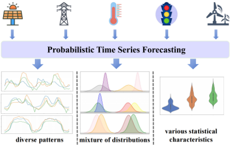
However, these methods struggle to accurately capture the intricate temporal dynamics and statistical properties of longterm time series. Given the perpetual evolution of economic, social, and environmental factors, time series data are prone to concept drift, which can diminish the performance of previously effective models in new contexts. As depicted in Figure 1, real-world time series data commonly displays diverse patterns, mixture of distributions, as well as various statistical characteristics, posing challenges for conventional methods to precisely capture such features. First, it is difficult to extract temporal patterns which are entangled and diversified. Second, the mixed distribution of data exacerbates the challenge of capturing probabilistic distribution information. Third, the diverse statistical properties of data complicate models' ability to simultaneously capture quantile information from multiple variates.
To tackle the aforementioned challenges, we propose a novel framework called QuantileFormer based on a patternmixture decomposition method for probabilistic time series forecasting. To depict the intricate temporal patterns and stochastic characteristics in time series data, we propose a pattern-mixture decomposition approach to decompose the long-term time series into different pattern components to facilitate analysis. Pattern-mixture decomposition is composed of two key components: drift-divergence and Gaussian mixture decomposition. The drift-divergence decomposition employs a quantile filter to break down the original time series into quantile drift and divergence pattern components, thereby enhancing the model's predictive power. Following this, Gaussian mixture decomposition is utilized to further decompose the divergence patterns into a blend of multiple Gaussian distributions. This step assigns probabilities to each data point, allowing the model to quantify the uncertainty associated with predictions by identifying which distribution each point belongs to. The Gaussian distribution components are then processed by a variational inference network, which extracts information about the overall statistical properties of the time series data. We further design a fusion Transformer architecture that integrates these pattern components holistically to form the final quantile predictions for probabilistic time series forecasting.
The contributions of this paper are summarized as follows.
- We propose a pattern-mixture decomposition method that decomposes long-term time series into quantile drift, divergence patterns, and Gaussian mixture components, which can effectively capture the intricate temporal patterns and stochastic characteristics in time series data.
- We propose a novel Transformer-based model called QuantileFormer for probabilistic time series forecasting. Based on pattern-mixture decomposition, the quantile drift part is proceeded by a Transformer encoder and the statistical patterns are captured by a Variational AutoEncoder (VAE) network, which are fed into a fusion Transformer to obtain the quantile prediction results.
- We conduct comprehensive experiments to rigorously assess the efficacy of our proposed method. In addition to employing conventional metrics, we introduce a new performance metric, cpaw (Coverage Probability with Normalized Averaged Width), specifically designed to quantify the precision of the predicted probabilistic intervals. Experimental results show that the proposed method consistently outperforms the baseline methods by a large margin and achieves state-of-the-art performance on six real-world benchmarks.
2 RelatedWork
2.1 Transformer-basedModels
Transformer-based models were widely used in time series forecasting. Pyraformer [Liu et al., 2022] proposed a novel pyramidal attention based Transformer to bridge the gap between capturing the long-range dependencies and reducing time and space complexity. PatchTST [Nie et al., 2022] used patch to provide a longer sequence of inputs to extract meaningful temporal relationships and channel independence to predict multivariate time series. iTransformer [Liu et al., 2023] encoded each variable as an independent token, and used the feedforward network to model the temporal correlation of variable variables to obtain better sequential temporal representation. However, the above mentioned works mainly focused on point-wise forecasting, and very few works adopted Transformer for probabilistic forecasting [Eisenach et al., 2020; Lim et al., 2019].
2.2 Decomposition of Time Series
In the realm of time series analysis, the standard methodology of time series decomposition [Cleveland et al., 1990; Tukey, 1960; Hyndman and Khandakar, 2008; De Jong, 1980; McCullough and Renfro, 1990] dissects a temporal sequence into several components, each representing a more predictably discernible underlying pattern. When applied to forecasting tasks, decomposition serves as an essential preprocessing step for historical series prior to predicting future sequences. Examples include the application of trendseasonality decomposition in models like Autoformer [Wu et al., 2021] and FeDFormer [Zhou et al., 2022], period decomposition in TimesNet [Wu et al., 2022], basis expansion in N-BEATS [Oreshkin et al., 2019], and matrix decomposition in DeepGLO [Sen et al., 2019]. TS3Net [Ma et al., 2024] expanded the time series into a 2D temporal-frequency distribution and decoupled a long-term series into trend-part, regularpart, and fluctuant-part. TimeMixer [Wang et al., 2024] extracted past information and blended seasonal and trend components at different scales separately.
2.3 Probabilistic Time Series ForecastingMethods
To capture the parts of the sequence that reflect the probability distribution, several methods have been applied to probabilistic time series forecasting [Bontempi and Ben Taieb, 1999; Hyndman and Athanasopoulos, 2018; Bergmeir and Hyndman, 2015; Salinas et al., 2018; Wang et al., 2021]. PTSE [Zhou et al., 2023] proposed a multi-model distribution ensemble method which abstracts the transformation of the model into Hidden Markov Model. Conformalized quantile regression [Romano et al., 2019] involved regressing the recentered influence function (RIF) of the quantile functional over input covariates to obtain unconditional quantile regression. TimeGrad [Rasul et al., 2021] proposed an autoregressive model for multivariate probabilistic forecasting that leverages the exceptional performance of EBMs to learn from the distribution of the next time step. TMDM [Li et al., 2024] took into account the covariate dependence of forward and reverse processes in the diffusion model to achieve highly accurate distribution estimation of future time series.
To the best of our knowledge, we are the first to propose a pattern-mixture method that decomposes long-term series into a mixture of quantile patterns, and design a fusion Transformer architecture for probabilistic time series forecasting.
3 ProblemFormulation
Probabilistic time series forecasting focuses on predicting the quantiles for each time point of a time series. Quantiles are essential statistical measures that provide insights into the distributional properties of a random variable. In the context of probability distributions, a quantile represents a critical value below which a specified proportion of the distribution lies. For a given probability p, the p-quantile is defined as the value xp such that P(X ≤ xp) = p, where X is a random variable and P denotes the probability measure. The quantile function, often denoted as Q(p), maps a probability p to the corresponding quantile xp, which is expressed as:
Considering the rolling forecasting setting with a fixed size window, we have the observations at T time points, represented by X = {xi|i = 1, 2, ...T}. The objective is to perform quantile regression for time series analysis, i.e., estimating the conditional quantiles of the response variable y at different percentiles τ , which can be expressed as:
where Xt denotes the vector of observed variables at time t; yt is the predicted quantile at time t; βt is the vector of coefficients for the τ-th quantile; and Qτ(yt|Xt) represents the τ -th conditional quantile of yt given Xt.
The quantile regression problem can be formulated as the following optimization problem:
where u = yt -Xtβτ is the residual for the t-th observation; ρτ(u) is the loss function that penalizes the residuals with respect to the τ-th quantile.
4 QuantileFormer Model
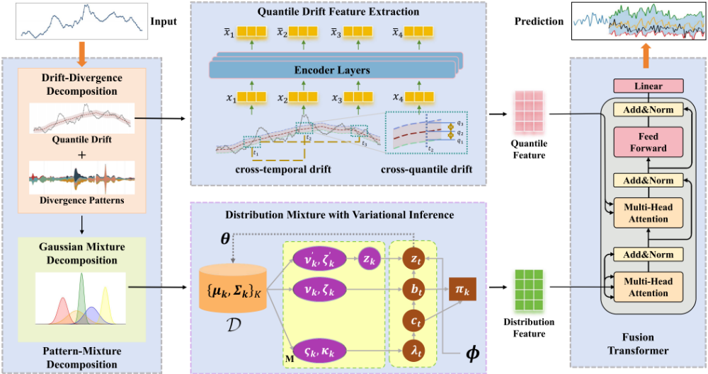
We propose a framework called QuantileFormer for probabilistic time series forecasting, which is illustrated in Figure 2. It begins with a pattern-mixture decomposition method, which meticulously breaks down long-term time series data into distinct pattern components to capture essential temporal dynamics. This decomposition process is composed of two main elements: a Drift-Divergence decomposition that isolates quantile drift and divergence patterns, and a Gaussian mixture decomposition that characterizes the global statistical properties of the data. These components provide a detailed description of the temporal and statistical features inherent in the time series. To further refine the analysis, we incorporate a quantile drift feature extraction module that adeptly extracts meaningful features from the quantile drift. Concurrently, a variational inference network is employed to deduce broader distributional insights from the divergence patterns. Finally, to synthesize the insights gained, we propose a fusion Transformer module, which fuses the pattern components to form the final quantile prediction results, thereby offering a comprehensive and robust approach for probabilistic time series forecasting.
4.1 Pattern-Mixture Decomposition
The pattern-mixture decomposition consists of two submodules: a drift-divergence decomposition and a Gaussian mixture decomposition, which are introduced as follows.
Drift-Divergence Decomposition
Conventional methods for sequence decomposition roughly separate the series into the trend-cyclical and seasonal parts. However, these two parts contribute little to quantile regression due to their nature of statistics. To this end, we propose a drift-divergence decomposition method to capture different quantile levels and complex composite patterns within the sequence, referring to as Quantile Drift and Divergence Patterns. For each quantile q in the quantile set Q, we extract the drift component χq of the original series using a sliding window. We use χQ to represent the set containing all the drift components, i.e., χQ = {χq }q∈Q. Specifically, for each q, we calculate the drift component χq and the divergence component χd as follow:
where χd denotes the divergence patterns obtained by subtracting the median χ0.5 from the original series χ; and QuantileF ilt(·, q) represents the moving q-th quantiles with padding operation to keep the series length unchanged.
Gaussian Mixture Decomposition
After drift-divergence decomposition, the quantile drift χQ represents smooth components of the time series, and the divergence component χd contains complex periodic patterns and distribution characteristics. We propose a Gaussian mixture decomposition method to further capture statistical patterns from the divergence component χd .
Gaussian Mixture Models (GMM) [Ng and Jordan, 2001] is a probabilistic model that represents a mixture of multiple Gaussian distributions. The probability density function for a single Gaussian distribution is:
where x is the data vector; µ is the mean vector; Σ is the covariance matrix; and d is the dimensionality of the data. We hope to find a set of Θ = {µk,Σk}k based on which the Gaussian distribution ensemble can optimally fit the divergence patterns χd . The probability of the set Θ given the divergence patterns χd can be denoted as:
GMM decomposition aims to maximize the above likelihood function, which can be achieved by an iterative optimization algorithm such as Expectation-Maximization. We use GauDe(·) to summarize the above operations. Thus, we have
where D = {µk, Σk}Kk=1 represents the K Gaussian components which optimally fits χd .
4.2 DistributionMixture Inference with Variational AutoEncoder (VAE)
Due to the intricate nature of data distribution, the local distributions do not linearly constitute the global distribution in a straightforward manner, thereby complicating the derivation of the target distribution. The Gaussian components D = {µk,Σk}Kk=1 conveys essential information about the local distribution of the time series. We use ˆD to denote the target global distribution which has K components:
where Dk is the kth Gaussian component and πk ≥ 0, ∑Kk=1 πk = 1. Note that each time step data can be allocated into some of the K components [Ioffe and Szegedy, 2015]. We further introduce the following notations to describe the model.
- ct ∈ {0, 1}K is a binary vector representing the distribution allocation, where ctk = 1 represents the distribution of the tth time step is allocated to the kthe Gaussian component.
- bt = {btk ∈ [0, 1]|k = 1, ...K}, subject to ∑Kk=1 btkctk = 1, represents the contribution of the tth time step which are hyperparameters in the proposed distribution inference network. Noted that the contribution btk ̸= 0 only when the corresponding allocation component ctk = 1.
Since the true distribution is unknown, we propose a Variational AutoEncoder (VAE) method to approximate the optimal parameters πk, ct and bt of the global distribution.
Using the stick-breaking construction of the Indian Buffet Process (IBP) [Griffiths and Ghahramani, 2011], we infer that ct is sampled from a Bernoulli distribution parameterized by λt = {λtk|k = 1, ...K}, where λt is sampled in i.i.d from a Beta distribution Beta(ςk, κk) parameterized by ςk, κk. Similarly, we infer that bt is sampled from a Gaussian prior distribution N(νk, ζk) which is parameterized by νk and ζk.
We denote zt = ∑Kk=1 btk ˙zt, which is a latent variable used by a variational decoder θ to reconstruct the given D. In the expression, zt means the latent vector sampled from every allocated distribution of tth time step from Gaussian prior distribution N(ν ′k , ζ ′k ), which can adaptively adjust the latent posterior to a suitable probabilistic distribution [Duan et al., 2023].
As illustrated in Figure 2, the parameters of Beta(ςk, κk), N(νk, ζk) and N(ν ′k , ζ ′k ) can be inferred with a variational encoder ϕ based on the Gaussian components D, i.e., {νk, ζk, ν ′k , ζ ′k , ςk, κk} = ϕ(D). Meanwhile, bt and zk contribute to the calculation of a latent variable zt, which is then fed to a decoder θ.
In order to infer the latent vector zt, we should derive the variational posterior qϕ(λt, ct, bt). From Figure 2 we know that variables in variational posterior are conditionally independent with the priori p(D). So we can decouple the variables as: qϕ(λ, c, b) = ∏Kk=1 ∏Mm=1 qϕ(btk) · qϕ(ctk|λtk) ·
qϕ(λtk), where the variational posterior distributions can be derived as[Cote, 2016]:
Given the model structure, the component weights πk can be inferred from the allocation vector ct and the contribution values bt. To derive the component weight πk, we use a softmax function[Dempster et al., 1977] over the expected contribution of each component across all time steps:
and Z is a normalization constant:
By optimizing the parameters, the optimal bt and ct can be derived, which can be further used to derived the distribution weights πk.
We then introduce the algorithm to optimize the VAE based on the derivation in the above section. For convenient, we omit the latent variables {bt, ct, λt} and their priors in representing the encoder model ϕ.
The true posterior pθ(zt|D) is typically intractable, thus we approximate it with qϕ(zt|D) .by minimizing their KLdivergence:
where
Since directly computing pθ(zt|D) is difficult, we optimize the ELBO (Evidence Lower BOund) [201, 2012].
According to the theory of variational inference [Kingma, 2013], the above problem can be solved with the SGD method using a nonlinear deep neural network to optimize the mean squared error loss function.
We summarize the above operation as VAE(·, ·). Thus, we can obtain indications of the global distribution by
which linearly projects each time point in χd onto a Gaussian distribution in D. The output χdout contains rich global distribution information providing insights into the shape, spread, and central tendency of the time series, which can facilitate the subsequent probabilistic time series forecasting task.
4.3 Quantile Drift Feature Extraction
The decomposed drift component χQ encapsulates a wealth of drift information within the sequence. Recognizing the heterogeneity in these drifts, we incorporate both cross-time drift and cross-quantile drift into our considerations. Crosstime drift captures temporal interactions between data at different time steps, while cross-quantile drift reveals disparities in trends across quantile levels.
We apply Transformer encoder on χQ to capture the drift features. The Transformer encoder consists of multiple identical layers (typically 6 layers). Each encoder layer consists of two sub-layers: a Multi-Head Self-Attention Layer and a Fully Connected Feedforward Layer. Residual connections and layer normalization are also included between these two sublayers. We use χeout = Encoder(χ) to represent the Transformer encoder. Thus we have χQeout = {Encoder(χq )}q∈Q to denote the encoder output of the quantile drift feature.
4.4 Fusion Transformer with Cross-Attention
To fuse the output features from different components to form the final prediction, we design a Fusion Transformer with cross-attention to establish a soft correspondence between the drift-divergence (i.e., χQeout and χdout ) , as illustrated in the right part of Figure 2. We first align χdout with χQeout using a linear projection W a . Then we adopt three linear projections WK , WQ, WV to generate the Query-Key-Value triples as follows.
We then apply cross-attention among Q, K, and V and following by a FeedForward Network (FFN) to enhance the expressive capability of the model. We highlight the core calculation process as:
where Att(·, ·, ·) is the multi-head attention module.
The residual connections allow the network to retain the original Gaussian mathematical implications, which contain quantile drift and Gaussian components information to enrich the final predictions. Thus the final output of prediction result is
where W is the parameter of the linear prediction head.
4.5 Loss Function
In order to synthesize the information of the context vectors, we train our model by combining the losses of three parts, and each part of the loss is measured by a quantile loss function. In line with previous works [Wen et al., 2017; Lim et al., 2019; Zhou et al., 2023], we use a jointly quantile loss which sums across all quantile outputs for horizons in the future, i.e., τ ∈ 1..., τmax, to train our model:
where Ω is the domain of training data containing M samples, Q is the set of output quantiles, and (·)+ = max(0, ·).
| ELECTRICITY | WIND | |||||||||
|---|---|---|---|---|---|---|---|---|---|---|
| 0.5 | 0.6 | 0.7 | 0.8 | 0.9 | 0.5 | 0.6 | 0.7 | 0.8 | 0.9 | |
| DEEPAR | 1.0002 | 1.1177 | 1.9544 | 1.2077 | 1.0830 | 1.0205 | 0.9987 | 0.7805 | 1.0182 | 1.4419 |
| MQRNN | 1.1648 | 1.5772 | 1.6336 | 1.8193 | 0.8273 | 2.1937 | 4.4670 | 5.5987 | 5.9560 | 1.8574 |
| TFT | 1.5547 | 1.0037 | 1.0440 | 0.8772 | 0.7618 | 0.9526 | 0.8611 | 0.7978 | 0.6568 | 0.4658 |
| TRANSFORMER | 1.3703 | 0.8873 | 1.0098 | 0.9005 | 0.9439 | 1.0011 | 1.0585 | 0.9898 | 0.9006 | 0.9750 |
| AUTOFORMER | 1.0584 | 0.9191 | 1.0301 | 0.8786 | 0.6420 | 1.4353 | 1.6054 | 1.3345 | 0.9921 | 0.6361 |
| FEDFORMER | 1.9429 | 1.0447 | 0.9669 | 3.0007 | 1.0618 | 1.1361 | 1.0831 | 1.2615 | 0.6544 | 0.3876 |
| PATCHTST | 1.8354 | 1.3134 | 1.0657 | 0.8800 | 0.7567 | 1.4666 | 0.9831 | 1.1394 | 0.9008 | 0.3667 |
| ITRANSFORMER | 1.3430 | 1.0348 | 1.2174 | 0.9072 | 1.2742 | 1.5983 | 1.0314 | 0.8091 | 0.6814 | 0.9900 |
| QUANTILEFORMER | 0.7469 | 0.8136 | 0.3330 | 0.4340 | 0.5121 | 0.8403 | 0.9105 | 0.7346 | 0.5842 | 0.3369 |
| ETTM1 | ETTH1 | |||||||||
| 0.5 | 0.6 | 0.7 | 0.8 | 0.9 | 0.5 | 0.6 | 0.7 | 0.8 | 0.9 | |
| DEEPAR | 1.2026 | 1.1749 | 0.7901 | 1.0616 | 0.5388 | 2.3414 | 0.7631 | 1.2217 | 1.0815 | 1.9889 |
| MQRNN | 16.5845 | 21.9918 | 17.9190 | 12.0559 | 3.6909 | 1.4757 | 1.6722 | 1.0317 | 1.1949 | 1.2239 |
| TFT | 0.4930 | 0.7829 | 0.6769 | 0.4976 | 0.3513 | 1.4639 | 1.0443 | 0.9283 | 0.7382 | 0.3662 |
| TRANSFORMER | 1.0397 | 0.8740 | 0.7372 | 0.4998 | 0.3618 | 1.1989 | 0.8805 | 0.7284 | 0.4868 | 0.5546 |
| AUTOFORMER | 1.8463 | 1.3424 | 1.1008 | 0.8392 | 0.4774 | 1.7221 | 1.2556 | 1.1977 | 0.9091 | 0.4569 |
| FEDFORMER | 0.6619 | 0.8673 | 0.4927 | 0.5491 | 0.3865 | 0.9480 | 0.8875 | 0.8328 | 0.7208 | 0.4582 |
| PATCHTST | 1.4268 | 1.3088 | 1.0240 | 0.5100 | 0.2816 | 1.4719 | 1.4558 | 1.1307 | 0.4275 | 0.3166 |
| ITRANSFORMER | 0.7514 | 0.4112 | 0.8834 | 0.5824 | 0.1228 | 0.8850 | 0.9508 | 0.8607 | 0.4721 | 0.3129 |
| QUANTILEFORMER | 0.1536 | 0.1642 | 0.2689 | 0.4340 | 0.0596 | 0.3007 | 0.6130 | 0.2912 | 0.4273 | 0.3388 |
| SOLAR | TRAFFIC | |||||||||
| 0.5 | 0.6 | 0.7 | 0.8 | 0.9 | 0.5 | 0.6 | 0.7 | 0.8 | 0.9 | |
| DEEPAR | 0.8666 | 1.1173 | 1.2854 | 1.4512 | 1.6117 | 1.0502 | 0.8813 | 1.2484 | 0.9394 | 1.1539 |
| MQRNN | 0.8994 | 1.3492 | 1.0459 | 1.1921 | 1.7157 | 1.8146 | 2.2111 | 2.5796 | 2.9482 | 0.9940 |
| TFT | 1.0039 | 1.1082 | 1.2493 | 1.3740 | 1.0015 | 1.1494 | 0.8900 | 0.8500 | 0.5862 | 1.0570 |
| TRANSFORMER | 1.0391 | 1.1617 | 1.1381 | 1.0794 | 1.0777 | 0.9664 | 0.9325 | 1.0574 | 0.8679 | 0.9247 |
| AUTOFORMER | 1.1641 | 1.2367 | 1.2088 | 1.0030 | 0.6167 | 0.9908 | 1.1109 | 0.8686 | 0.6064 | 0.4970 |
| FEDFORMER | 1.0363 | 1.1708 | 1.0261 | 1.5427 | 0.6414 | 2.4497 | 0.9188 | 2.3784 | 1.7356 | 0.8770 |
| PATCHTST | 1.0806 | 1.1242 | 1.2547 | 1.1935 | 0.5950 | 0.9775 | 1.6937 | 1.1269 | 0.5962 | 1.1450 |
| ITRANSFORMER | 1.0705 | 1.1843 | 1.1845 | 1.3705 | 1.6083 | 1.8998 | 1.3545 | 1.1941 | 0.8247 | 1.5621 |
| QUANTILEFORMER | 1.0641 | 1.0480 | 1.1832 | 1.0008 | 0.5883 | 0.8489 | 0.8291 | 0.8489 | 0.5998 | 0.4688 |
| DATASET | RANGE | FREQ | SAMPLES | FEATURES |
|---|---|---|---|---|
| ELECTRICITY | 2016/7/1 TO 2019/7/1 | 1H | 26304 | 321 |
| ETTM1 | 2016/7/1 TO 2018/6/26 | 15MIN | 69680 | 7 |
| ETTH1 | 2016/7/1 TO 2018/6/26 | 1H | 17420 | 7 |
| WIND | 2020/7/1 TO 2023/2/28 | 15MIN | 93412 | 3 |
| TRAFFIC | 2016/7/1 TO 2018/7/2 | 1H | 17544 | 861 |
| SOLAR | 2020/1/1 TO 2023/1/31 | 15MIN | 108192 | 5 |
| ELEC. | WIND | ETTM1 | ETTH1 | TRAFFIC | SOLAR | |
|---|---|---|---|---|---|---|
| DEEPAR | 5.2890 | 5.4470 | 3.8999 | 8.6446 | 4.8742 | 11.2021 |
| MQRNN | 3.8166 | 2.8071 | 8.4531 | 5.2274 | 1.6137 | 5.6390 |
| TFT | 2.0002 | 2.4662 | 2.6199 | 2.1166 | 3.0367 | 1.7246 |
| TRANSFORMER | - | - | 0.8988 | - | - | 2.3645 |
| AUTOFORMER | 3.2389 | 3.2790 | 1.8055 | 1.8830 | 2.3327 | 4.2420 |
| FEDFORMER | 2.3841 | 2.1214 | 3.7312 | 1.1557 | 2.8512 | 2.1066 |
| QUANTILEFORMER | 1.9902 | 1.8435 | 5.0815 | 4.4471 | 1.5858 | 0.8335 |
5 Experiments
Datasets: We evaluate the performance of our proposed model based on the following open datasets: (1) Electricity, (2) ETT [Zhou et al., 2020], which contains four subsets ETTm1, ETTm2, and ETTh1, and ETTh2, (3) Traffic, (4) Solar, (5) Wind. Information are shown in Table 2.
Baselines We compare the proposed QuantileFormer with three state-of-the-art probabilistic forecasting models, which include TemporalFusionTransformer (TFT) [Lim et al., 2019], DeepAR [Salinas et al., 2020] and MQRNN [Wen et al., 2017]. We also compare our model with other Transformer-based models, such as PatchTST [Nie et al., 2022], iTransformer [Liu et al., 2023], Autofomer [Wu et al., 2021], FeDformer [Zhou et al., 2022] and Transformer [Vaswani et al., 2017]. Note that the later five Transformer-based models were designed for point-wise forecasting and we adapt them to quantile prediction by training them with the proposed quantile loss.
Performance Metrics: Previous works [Salinas et al., 2020] widely used the q-risk to quantify the accuracy of a q-th quantile of the predictive distribution, which is defined as:
where (·)+ = max(0, ·).
Since q-risk only considers the accuracy of quantiles, it is lack of consideration to measure the probabilistic interval (PI). To this end, we propose a new performance metric to measure how the true value interact with the predicted probabilistic interval. We combine the coverage probability with normalized averaged width to form the metric called cpaw, which is formulated by the PI coverage probability (PICP) and PI normalized averaged width (PINAW) as
where PICP = 1n ∑ni=1 I(yi ∈ [ˆ qi,l, ˆ qi,u]) calculates the average probability of whether an observation is within the prediction interval of corresponding quantile across all samples; PINAW = 1n |ˆ qi,u - ˆ qi,l| calculates the average percentage of the prediction interval width relative to the range of observations across all samples; µ represents the difference between the upper and lower quantiles; and γ is an indicative function reflecting whether the PICP exceeds µ.
| ELECTRICITY | WIND | |||||
|---|---|---|---|---|---|---|
| 0.5 | 0.7 | 0.9 | 0.5 | 0.7 | 0.9 | |
| W/O D-D DECOMP. | 0.7629 | 0.8890 | 0.6738 | 1.0746 | 1.2476 | 1.7182 |
| W/O GMM DECOMP. | 0.9890 | 0.9125 | 0.5570 | 0.9782 | 0.9575 | 0.4451 |
| W/O FUSION TRANSFORMER. | 0.9389 | 0.9104 | 0.9885 | 0.8954 | 0.8861 | 1.0460 |
| QUANTILEFORMER | 0.7546 | 0.3330 | 0.5121 | 0.8403 | 0.7346 | 0.3369 |
| SOLAR | TRAFFIC | |||||
| 0.5 | 0.7 | 0.9 | 0.5 | 0.7 | 0.9 | |
| W/O D-D DECOMP. | 1.3440 | 1.2463 | 0.6142 | 0.9626 | 1.3814 | 0.5497 |
| W/O GMM DECOMP. | 1.0831 | 1.1991 | 0.7914 | 1.3995 | 0.8849 | 0.5837 |
| W/O FUSION TRANSFORMER. | 1.0708 | 1.1930 | 0.7289 | 1.5161 | 1.1245 | 0.8275 |
| QUANTILEFORMER | 1.0641 | 1.1832 | 0.5883 | 0.8489 | 0.8489 | 0.4688 |
5.1 Main Results
Comprehensive forecasting results evaluated by q-risk are listed in Table 1 with the best in bold. We compare the experimental results at various quantile levels. The results show that QuantileFormer achieves the best performance in most cases, with an average q-risk decrease of 24% for 0.5 quantile, decrease of 15% for 0.6 quantile, decrease of 27%, 14%, and 22% for 0.7, 0.8, and 0.9 quantile respectively, compared to the second-place algorithm.
Performance evaluated by cpaw is shown in Table 3. By analyzing the table, we make the following discussions and conclusions. 1) Compared with methods which are based on Transformer (i.e., TFT, Transformer, Autoformer, FeDformer, PatchTST and iTransformer), our method achieves 20% and 51% improvement on Wind and Traffic dataset, respectively. 2) Compared with methods which are based on RNN (i.e., DeepAR, MQRNN), our method improves by 55%, 50% and 88% on Electricity, Wind and Traffic datasets over other baselines, respectively.
5.2 Ablation Study
To explore the role of each module in our proposed framework, we compare the prediction results obtained by different sections as shown in Table 4. In the results, removing each component results in performance drop in different levels, showcasing the effectiveness of the proposed framework. We conduct experiments without the drift-divergence decomposition, the Gaussian mixture model decomposition and the fusion Transformer module respectively.
5.3 Hyperparameters Analysis
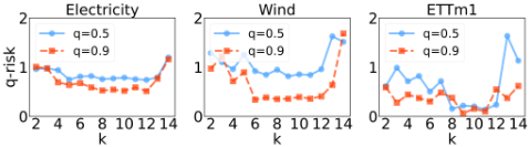
We analysis the impact of hyperparameters. i.e., selection of the number of Gaussian components k on the model's final performance, and the results are illustrated in Figure 3. According to the figure, if k is too small (e.g., k ≤ 4), the performance is relative poor due to no enough Gaussian components to describe the mixture distribution. If k is too large (e.g., k ≥ 12), the performance also degrade, probably due to overfitting. A suitable k is within [8,10] for Electricity, within [6,10] for Wind, and within [8,11] for ETTm1.
5.4 Visualization
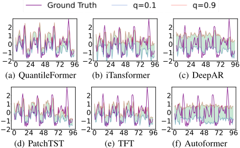
We visualize the probabilistic forecasting results of different models as in Figure 4 (the Electricity dataset). These visualizations offer insights into how different models perform in capturing the underlying uncertainty and predictive trends within each respective dataset. It demonstrates that the QuantileFormer is more in line with the ground truth, with a much narrower probabilistic interval (PI) and a lower q-risk. This verify the effectiveness of the pattern-mixture decomposed Transformer model.
6 Conclusion
This paper introduced QuantileFormer, a novel Transformerbased model that revolutionizes probabilistic time series forecasting through a meticulous pattern-mixture decomposition approach. It decomposed complex time series data into quantile drift and divergence patterns, capturing the nuanced temporal dynamics and stochastic features. The quantile drift was captured by an encoder, while the divergence patterns were broken down into Gaussian mixture components. A Variational distribution inference network was introduced to extract the global statistical properties. These decomposed elements were then merged by a fusion Transformer, which synthesizes the information to produce accurate quantile predictions. Through extensive experimentation, the paper demonstrated the efficacy of the proposed model, confirming its effectiveness in probabilistic time series forecasting.
Acknowledgments
This work was partially supported by the Natural Science Foundation of Jiangsu Province (Grant No.BK20222003), the Collaborative Innovation Center of Novel Software Technology and Industrialization, and the Sino-German Institutes of Social Computing. The corresponding author is Wenzhong Li (lwz@nju.edu.cn).
@inproceedings{ijcai2025p684,
  title     = {QuantileFormer: Probabilistic Time Series Forecasting with a Pattern-Mixture Decomposed VAE Transformer},
  author    = {Shao, Yimiao and Li, Wenzhong and Xia, Kang and Lin, Kaijie and Lin, Mingkai and Lu, Sanglu},
  booktitle = {Proceedings of the Thirty-Fourth International Joint Conference on
               Artificial Intelligence, {IJCAI-25}},
  publisher = {International Joint Conferences on Artificial Intelligence Organization},
  editor    = {James Kwok},
  pages     = {6147--6155},
  year      = {2025},
  month     = {8},
  note      = {Main Track},
  doi       = {10.24963/ijcai.2025/684},
  url       = {https://doi.org/10.24963/ijcai.2025/684},
}
TY - CPAPER TI - QuantileFormer: Probabilistic Time Series Forecasting with a Pattern-Mixture Decomposed VAE Transformer AU - Shao, Yimiao AU - Li, Wenzhong AU - Xia, Kang AU - Lin, Kaijie AU - Lin, Mingkai AU - Lu, Sanglu T2 - Proceedings of the Thirty-Fourth International Joint Conference on Artificial Intelligence, IJCAI-25 PB - International Joint Conferences on Artificial Intelligence Organization PY - 2025 SP - 6147 EP - 6155 DO - 10.24963/ijcai.2025/684 UR - https://doi.org/10.24963/ijcai.2025/684 ER -Copied
Machine-readable versions of this paper, for tools and AI agents:





