
A Symmetric Relative-Error Loss Function for Intermittent Multiscale Signal Modelling
Proceedings of the Thirty-Fourth International Joint Conference on Artificial Intelligence. Main Track. Pages 6281-6288.
https://doi.org/10.24963/ijcai.2025/699
Keywords
- Machine Learning: ML: Supervised Learning
- Machine Learning: ML: Optimization
- Machine Learning: ML: Time series and data streams
- Machine Learning: ML: Regression
Abstract
Multiscale signals represent a formidable modelling challenge in Machine Learning as the ubiquitous Mean Squared Error loss function neglects signal behaviour at smaller values. Several scale-equalizing error metrics have been devised to tackle this problem, amongst which the Mean Absolute Percentage Error (MAPE) remains the most widely used due to its simplicity and interpretability. However, by its very definition, MAPE introduces three major issues: asymptotic behaviour at zero-target values, asymptotic gradient behaviour at zero error, and accuracy loss for large signal scales. We address these limitations by proposing the Symmetric Mean Arctangent Squared Percentage Error (SMASPE), which builds up from the Mean Arctangent Absolute Percentage Error (MAAPE) and leverages a mathematically smoother definition along with user-provided signal bounds to extend its functionality. The numerical properties of SMASPE are explored, and its performance is tested in two real-life cases for deterministic and stochastic optimization. The experiments show a clear advantage of the proposed loss function, with an improvement of up to 42% with respect to MAAPE in terms of Mean Absolute Error for deep learning models when appropriate bounds are selected.
- [Bradbury et al., 2018] James Bradbury, Roy Frostig, Peter Hawkins, Matthew James Johnson, Chris Leary, Dougal Maclaurin, George Necula, Adam Paszke, Jake VanderPlas, Skye Wanderman-Milne, and Qiao Zhang. JAX: compos- able transformations of Python+NumPy programs, 2018.
- [Cho, 2014] Kyunghyun Cho. Learning phrase representa- tions using rnn encoder-decoder for statistical machine translation. arXiv preprint arXiv:1406.1078, 2014.
- [Chollet and others, 2015] Franc ¸ois Chollet et al. Keras. https://keras.io, 2015. Link
- [De Myttenaere et al., 2016] Arnaud De Myttenaere, Boris Golden, Bénédicte Le Grand, and Fabrice Rossi. Mean absolute percentage error for regression models. Neuro- computing, 192:38-48, 2016.
- [Henderson, 1975] Charles R Henderson. Best linear unbi- ased estimation and prediction under a selection model. Biometrics, pages 423-447, 1975.
- [Hodson et al., 2021] Timothy O Hodson, Thomas M Over, and Sydney S Foks. Mean squared error, decon- structed. Journal of Advances in Modeling Earth Systems, 13(12):e2021MS002681, 2021.
- [Hyndman and Koehler, 2006] Rob J Hyndman and Anne B Koehler. Another look at measures of forecast accuracy. International journal of forecasting, 22(4):679-688, 2006.
- [Kim and Kim, 2016] Sungil Kim and Heeyoung Kim. A new metric of absolute percentage error for intermittent demand forecasts. International Journal of Forecasting, 32(3):669-679, 2016.
- [Legendre, 1806] Adrien Marie Legendre. Nouvelles méthodes pour la détermination des orbites des comètes: avec un supplément contenant divers perfectionnemens de ces méthodes et leur application aux deux comètes de 1805.
- Courcier, 1806.
- [Liano, 1996] Kadir Liano. Robust error measure for super- vised neural network learning with outliers. IEEE Transac- tions on Neural Networks, 7(1):246-250, 1996.
- [Steinhauser, 2016] Martin Steinhauser. Computational mul- tiscale modeling of fluids and solids. Springer, Berlin, Germany, 2 edition, December 2016.
- [Vanegas Arias, 2025] Sergio Mauricio Vanegas Arias. A symmetric relative-error loss function for intermittent mul- tiscale signal modelling (github repository). https://github. com/sergiovaneg/SMASPE, 2025. Accessed: 2025-05-29. Link
- [Veera, 2020] Pearl Veera. Weekly sku level product sales transactions. https://www.kaggle.com/datasets/pearlveera/ weekly-sku-level-product-sales-transactions, 2020. Link
References were extracted automatically from the PDF and may contain errors.
Full text extracted automatically from the PDF; figures, tables and equations may differ. The PDF is the version of record.
1 Introduction
When performing regression tasks, regardless of context or modelling technique, the most common way to determine the fitness of a model is to calculate the Mean Squared Error (MSE). First described in [Legendre, 1806] as an algebraic procedure for fitting linear equations to data and later proven to be optimal for the lowest-sampling-variance estimator under unbiased assumptions [Henderson, 1975], it has persisted as the go-to loss function in the field of Machine Learning (ML) due to its context-free nature and, more importantly in the context of back-propagation, function smoothness. Unfortunately, this generality renders the MSE unsuitable for measuring model fitness when the sample space is not normally distributed or signal outliers are significant [Liano, 1996]. Such is the case of multiscale modelling problems, amongst which physical models such as the Navier-Stokes equation [Steinhauser, 2016] or intermittent signal forecasts like that of Photo-Voltaic (PV) energy generation can be mentioned.
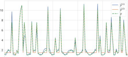
To illustrate the problems associated with minimizing the MSE for multiscale spaces, a synthetic example is presented: let y be the target signal defined by
where each βi is a sample drawn from a single-trial Binomial distribution with a 0.15 probability of success. Two dynamical system estimators, namely ˆy(1) and ˆy(2) , are defined as
The first estimator introduces multiplicative noise to the reference signal. In contrast, the second one perfectly captures the peaks introduced by the intermittent signal β while holding the constant that minimizes the squared error in its absence. Simulating these conditions yields the curves shown in Figure 1a and MSEs of 0.215 and 0.107 for estimators 1 and 2 respectively, which empirically evidences how this metric mathematically neglects small-scale dynamics.
In ML regression, the traditional way to cope with these variations in scale is to fit the models to minimize the Mean Absolute Percentage Error (MAPE) [De Myttenaere et al., 2016], defined as
where ¯ δi := yi-ˆ yi yi is a term henceforth referred to as relative sample error.
The MAPE divides each sample's error by its target value, making errors at lower scales numerically comparable to those of larger reference magnitude. Figure 1b illustrates the equalization effect of this approach, with the MAPE of the
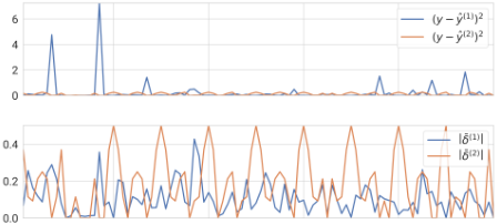
- (b) Squared and Relative Errors as perceived by the loss functions.
Figure 1: Synthetic multiscale example (100-sample window).
noisy signal now halving that of the small-scale-smoothing one (0.113 and 0.199 respectively). This effectively means a model trained to minimize the MAPE would better capture the behaviour of the signal. Unfortunately, the instability of this approach quickly becomes self-evident, since ∣∣¯ δ∣∣ → ∞ as |y| → 0 save for a perfect prediction, and even then stability cannot be guaranteed due to quantization.
Division by 0 is not uncommon in informatics and mathematical analysis, and some standard approaches have been proposed to handle this exception for regression applications [Hyndman and Koehler, 2006; Hodson et al., 2021]. However, [Kim and Kim, 2016] took an unconventional approach by interpreting ¯ δ as the hypotenuse slope of the "right triangle" defined by the perpendicular sides |y - ˆ y| and |y| to introduce Mean Arctangent Absolute Percentage Error (MAAPE), which measures the average angle of this slope as
Albeit a clever solution to the asymptotic behaviour at |yi| → 0+, choosing to preserve the absolute value of this ratio as a loss function introduces unwanted gradient behaviour at ˆ yi → yi. A smoother gradient can thus be attained by relaxing this one-to-one correspondence with the MAPE slope. Furthermore, by exploiting enforceable bounds, we can extend the definition to better capture the peak values of the signal without losing the small-scale dynamics.
This work modifies MAAPE and uses this extension as a functional unit to formulate the Symmetric Mean Average Squared Percentage Error (SMASPE). The specific contributions presented in this paper are the following:
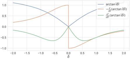
Figure 2: Sample-wise behaviour of the MAAPE and its first two derivatives as a function of the error ratio.
- The formulation of Mean Arctangent Squared Percentage Error (MASPE), a quadratic-relative-error variation of the MAAPE, and an analytical study of the mathematical properties that render it a more suitable loss function for gradient-based optimization.
- SMASPE, a symmetrical extension of the MASPE that exploits heuristic signal bounds to allow models to capture multiscale dynamics, and a graphical study of its behaviour as a function of the predicted and reference signal values.
- A numerical validation of SMASPE's adequacy for deterministic and stochastic optimization algorithms.
The remainder of this paper is organized as follows. In Section 2, the benefits and drawbacks introduced using the above ratio's square instead of its absolute value are explored as a function of the auxiliary variable ¯ δ. Section 3 presents the symmetric bound-enforcement and studies its implications as a function of the reference and predicted values y and ˆ y. In Section 4, two real-world examples are used to showcase the capabilities of SMASPE. Finally, in Section 5, a summary of the obtained experimental results and possible extensions to the proposed methodology are laid out.
The code and complementary material is made available as a GitHub repository at [Vanegas Arias, 2025].
2 Unidimensional Analysis: Improvements over MAAPE
Figure 2 illustrates the MAAPE and its derivatives as functions of ¯ δ, with the first derivative being multiplied by -1 to highlight the direction of minimization. As mentioned in Section 1, optimizing the absolute value of this ratio makes this function C 0 (not continuously differentiable) over the real domain, which means it presents asymptotic behaviour at the origin and thus renders the optimization problem numerically unstable. This is the same phenomenon encountered when using the Mean Absolute Error (MAE) as a loss function, which makes the MSE better suited as a minimization target even if the MAE is being used as the main performance metric.
By loosening the trigonometrical correspondence with the MAPE and focusing on the utility of MAAPE as a minimization target, the equivalent MASPE can be derived from Equation (5), yielding
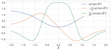
Since the arctangent is monotonically increasing, the predictor ˆy that minimizes MASPE for a given reference y also minimizes MAAPE. However, unlike its absolute-valued counterpart, Equation (6) belongs to C∞ (proof in complementary material) over the real domain. Thus, its gradient lacks MAAPE's discontinuity at the origin and, consequently, its second derivative is no longer asymptotic at 0 error, as shown in Figure 3.
It is worth noting that the price the MAAPE (and by extension the MASPE) pays for its boundedness is the vanishing gradient at infinity. Indeed, in both Figures 2 and 3 it is evident how the loss functions converge to π/2 as ¯ δ → ±∞, making its derivative converge to 0 by consequence. However, as shown in Section 3, this issue can be mitigated by enforcing loss-function symmetry w.r.t. known signal bounds.
3 Bidimensional Analysis: Symmetric Bounds
If by minimizing the expected squared error the MSE neglects small-scale system dynamics, then the relative-error approaches reviewed so far suffer an equivalent loss of accuracy at larger scales. Referring back to the synthetic example presented in Equation (1), the estimator defined by Equation (2) would be perceived to be twice as accurate as the one detailed in Equation (3) by the ¯ δ-based loss functions (MASPE included) despite consistently failing to capture the peak values of the intermittent signal. Therefore, an extension of the metrics explored so far that considers the behaviour of the loss as a function of both y and ˆ y is required.
Even if a system's dynamics are unknown, its domain can often be either characterized or empirically determined from data and thus be exploited to equalize measurable outputs reliably. Looking at the MASPE as a bidimensional function of y and ˆ y, let [y-, y+] ⊂ R be a real, finite interval bounding the target signal; i.e., -∞< y- ≤ yi ≤ y+ <∞ ∀i. Then, loss symmetry is enforced w.r.t. these bounds as
thus defining the SMASPE. Since this modification is merely the sum of two smooth functions evaluated on shifted (inverted) versions of the original signals y and ˆ y, the differentiability is preserved.
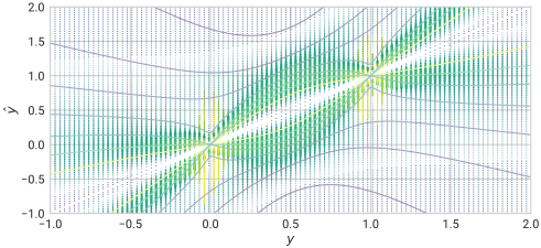
The second term of the above equation inverts the signal w.r.t. y+ so that large-scale dynamics are perceived as smallscale ones and vice versa. This effectively yields a numerically stable loss function within the user-defined interval, as illustrated by Figure 4, preventing the vanishing error gradients towards the upper bound of the modelled signal.
The [y-, y+] interval can be loosened as
where ∆y := y+ - y- and γ is a relaxation coefficient. This mitigates SMASPE's asymptotic behaviour near the symmetry bounds, further increasing the robustness of the approach. However, if overdone, the function may lose track of the difference in scale over the signal range, forfeiting the advantages of the relative-error approach. As evidenced by the vector field intensity in Figure 4, the trade-off SMASPE makes for its stability and domain coverage is its reliance on carefully defined bounds, which should follow a user-defined heuristic.
4 Applications
This section showcases the performance and versatility of the SMASPE with two real-life datasets. In Section 4.1, a comparative study for the real-life application presented in [Kim and Kim, 2016], Stock-Keeping Unit (SKU)-demand forecasting, is performed to illustrate the characteristics of SMASPE w.r.t. the State-of-the-Art (SotA). Then, in Section 4.2, a Deep Neural Network (DNN) is trained to forecast PV-generation using the SMASPE to highlight the advantages of the proposed loss function in backpropagation. In both experiments, the SMASPE is tested using tight and loose bounds (γ = 0.1, sensitivity analysis in complementary material).
The experiments were implemented in Python using the Jax [Bradbury et al., 2018] and Keras 3 [Chollet and others, 2015] stacks for ML model construction and training.
4.1 BFGS Optimization: Stock-Level Next-Sample Forecasting
As the first experiment, the performance of the loss functions proposed in this paper was tested for the same use-case studied in [Kim and Kim, 2016]. The experiments in this section were carried out using a Kaggle dataset [Veera, 2020] which, to the authors' knowledge, is the only open-access dataset sampled with the same frequency (i.e., weekly) and containing approximately the same number of samples per sequence as the one used for the original MAAPE paper.
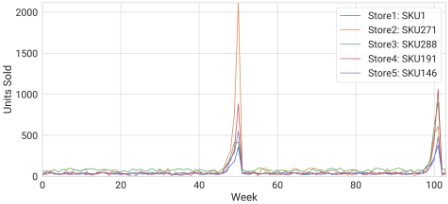
The dataset comprises 6000 time series, each containing 103 samples, representing the weekly sales volume per product across five retail stores, with one example from each of them being shown in Figure 5. Although not confirmed by the dataset description, it is reasonable to infer that the two sales peaks, approximately one year apart from each other, correspond to the sales near the holiday season, which explains the signal synchronization. Following the methodology of the MAAPE proposers [Kim and Kim, 2016], the first 95 samples were used to fit the models and the remaining 8 to evaluate their out-of-sample performance.
The considered models were the worst and best performers in [Kim and Kim, 2016]; namely, non-seasonal AutoRegressive Integrated Moving Average (ARIMA) and HoltWinters (HW) additive method (Triple Exponential Smoothing), respectively. Considering the length of the dataset, and since the authors did not provide the model parameters, a (4, 1, 4) order ARIMA and a HW with seasonality 4 were fitted separately to each time series, initializing the ARIMA model weights to 0 and the convex sum coefficients of the HW method to 0.5. These weights were adjusted by minimizing the MSE, MAAPE, MASPE, and SMASPE 1 . The performance of the fitted models was evaluated using all loss functions tested, the MAE, and their median convergence time (measured in iterations) in all sequences.
Table 1 contains the numerical results of the described experimental pipeline evaluated over the saturated model outputs, since negative demand values are not valid. From these results, the following can be stated:
- Despite the HWmodel converging generally faster than the ARIMA due to its lower parameter count (3 for HW vs. 10 for ARIMA), the previously worst-performing
1 Tight bounds set to each sequence's extrema.
(a) ARIMA model.
(b) HW model.
Figure 6: SKU demand model error distribution boxplots.
architecture ends up being the most accurate according to all error metrics when fitted using the SMASPE with moderately loose bounds. This, however, comes at an evident cost in convergence speed, requiring the most iterations out of all evaluated model-loss configurations.
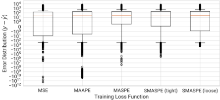
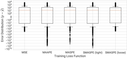
- Figure 6 provides some insight on MAAPE's poor performance for training the HWmodels. Indeed, despite all loss functions producing a similar distribution box, the MAAPE yields significantly more outliers of larger magnitude than the MSE or the loose SMASPE, explaining the difference in order of magnitude for the metrics in Table 1. This phenomenon could remain hidden for a small sample size, which might explain why the results in this paper contradict those of [Kim and Kim, 2016].
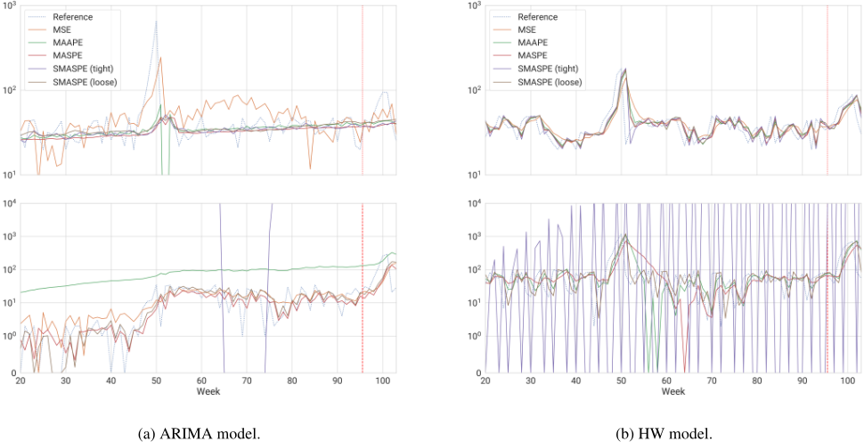
- Finally, even when performing numerically similar (on average) to its loose counterpart while converging significantly faster, the worst-case scenarios in Figure 7 illustrate how tight bounds for the SMASPE often lead to unstable model weights. This pathological behaviour makes itself numerically evident through the MAE and MSE metrics for the HWmodel.
4.2 Backpropagation: PVGeneration 3-Day-Ahead Forecasting
The second dataset is the PV energy generation. It comprises 821 full days (after clean-up) of hourly-sampled floating-point data including timestamps, weather measurements, and average generated power in kilowatts. Furthermore, the output signal was normalized from 0 to ∼ 1 by dividing each daily curve over the median peak of the 15 preceding days to avoid numerically neglecting generation values during low-sunlight seasons such as winter and prolonged storms, thus setting a heuristic for the SMASPE bounds.
| Model Loss | Median Iteration | Error Metrics (Out-of-Sample) | |||||
|---|---|---|---|---|---|---|---|
| Function | Number | MAE | MSE | MAAPE | MASPE | SMASPE (tight) | SMASPE (loose) |
| MSE | 23 | 4.32×10⁷ | 6.70×10¹⁸ | 0.648 | 0.554 | 1.07 | 0.653 |
| MAAPE | 5 | 3.19×10⁸ | 2.79×10¹⁸ | 0.638 | 0.562 | 1.13 | 0.700 |
| MASPE | 28 | 4.66×10³ | 9.43×10¹⁰ | 0.575 | 0.486 | 1.03 | 0.630 |
| ARIMA SMASPE (tight) | 9 | 3.09×10² | 1.62×10⁷ | 0.608 | 0.527 | 1.07 | 0.657 |
| SMASPE (loose) | 43 | 2.08×10² | 2.25×10⁵ | 0.528 | 0.429 | 0.934 | 0.553 |
| MSE | 2 | 2.31×10² | 2.35×10⁵ | 0.614 | 0.522 | 1.00 | 0.636 |
| MAAPE | 3 | 8.12×10⁴ | 2.97×10¹³ | 0.638 | 0.543 | 1.03 | 0.712 |
| MASPE | 5 | 8.78×10³ | 6.93×10¹¹ | 0.620 | 0.519 | 1.00 | 0.688 |
| HW SMASPE (tight) | 4 | 1.79×10⁵ | 2.68×10¹⁴ | 0.637 | 0.543 | 1.03 | 0.716 |
| SMASPE (loose) | 4 | 2.32×10² | 2.53×10⁵ | 0.558 | 0.441 | 0.912 | 0.614 |
Missing samples in the dataset impose a natural division that was used to determine the training, validation, and test partitions, resulting in a 59.1/29.7/11.2% scheme. In addition to the historical PV generation signal, global radiation and air temperature measurements were used as exogenous features, the forecasts of which can be retrieved during deployment and used as additional inputs. Since only the historical measurements of weather variables were logged, forecast uncertainty was simulated by introducing additive noise with exponentially increasing variance; namely,
where σx denotes the variance of the original variable x, ς represents the standard deviation of the white noise for the first sample over the prediction horizon, and β sets the exponential growth factor of the noise variance as a function of the sample index over the prediction horizon. These parameters were calibrated to ensure that the noise had a standard deviation of 0.1% of each feature's standard deviation at the beginning of the forecast horizon and increased tenfold by the end of the forecast window (i.e. β = ln 10 71 ).
The chosen architecture was an encoder/decoder Recursive Neural Network (RNN) with Gated-Recurrent Unit (GRU) layers similar to the scheme proposed by [Cho, 2014] with its hyperparameters fixed (1737 weights in total) for 72-hour context and forecast windows. The weights were randomly initialized five times and used as common starting points for all loss functions considered in Section 4.1, keeping the weights that achieved the median validation loss. These were minimized using the Adam optimizer (Learning Rate of 5 × 10⁻⁴ , 64 sequences per batch) for a maximum of 2000 epochs (500 patience epochs). Finally, rather than the actual extrema of the training partition, the expected [0, 1] interval was used to define the tight bounds.
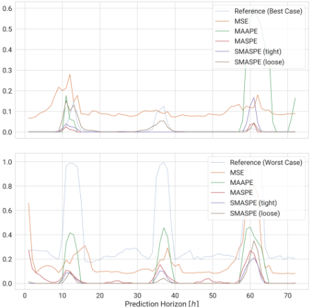
Table 2 contains the numerical results of the described experimental pipeline evaluated on the saturated model outputs, since negative generation values are not possible in this scenario. Figure 8 showcases the best and worst-case PVgeneration forecasts based on the IAE for the displayed pre-
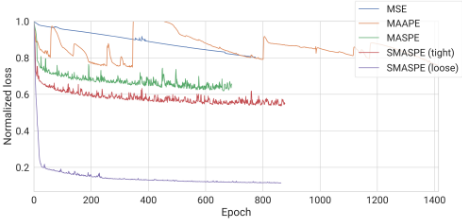
- (a) Loss history for the training partition (unsaturated output signal to avoid gradient clipping).
- (b) Loss history for the validation partition (saturated output signal).
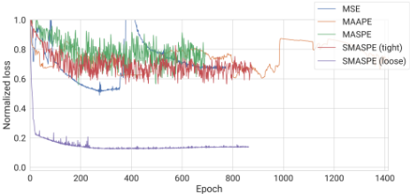
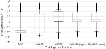
Figure 10: PV-generation model error distribution boxplots.
diction horizon. From these, the following can be stated:
- Despite the MSE and MAAPE converging the fastest out of all considered loss functions, Figure 9b reveals that this is due to the divergence of the validation loss. Since the MASPE history does not exhibit the same behaviour, it can be inferred that this issue stems frommodel overfitting and gradients around zero-relative-error respectively. This makes the models trained using the fast-converging loss functions perform significantly worse than the proposed ones for all error metrics evaluated over the test partition, as illustrated by Figure 8.
- On the opposite end of the spectrum, and as shown in Figure 9, MASPE models take the longest to converge due to the vanishing gradients brought up in Section 2.
| Median Epoch | Error Metrics (Testing Partition) | ||||||
|---|---|---|---|---|---|---|---|
| Loss Function | Number | MAE | MSE | MAAPE | MASPE | SMASPE (tight) | SMASPE (loose) |
| MSE | 774∗ | 0.179 | 0.143 | 1.13 | 1.15 | 1.28 | 0.649 |
| MAAPE | 855 | 0.185 | 0.132 | 0.901 | 0.866 | 1.02 | 0.550 |
| MASPE | 1050 | 0.123 | 0.121 | 0.726 | 0.655 | 0.786 | 0.243 |
| SMASPE (tight) | 974 | 0.109 | 9.79×10⁻² | 0.729 | 0.661 | 0.779 | 0.223 |
| SMASPE (loose) | 904 | 0.107 | 9.25×10⁻² | 0.715 | 0.641 | 0.756 | 0.215 |
Furthermore, Figure 10 reveals all proposed loss functions converge towards similar error distributions, yet the loose SMASPE remains the clear winner in terms of convergence speed and stability.
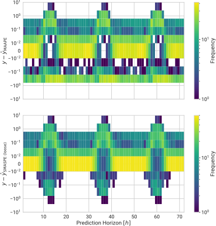
- The numerical results in Table 2 validate the increase in accuracy achieved by SMASPE, yielding relative improvements of 42% and 13% in terms of MAE w.r.t. MAAPE and MASPE-trained models respectively. Moreover, Figure 11 provides further insight into the signederror behaviour: while the MAAPE-trained model fails at capturing PV-generation peaks, the relaxed SMASPEtrained one achieves a near-symmetrical distribution at these critical points over the prediction horizon.
5 Conclusion
We have proposed the Mean Arctangent Squared Percentage Error (MASPE) as an improvement over MAAPE to prevent the asymptotic behaviour of the gradient at zero relative error. Moreover, we have proposed a novel loss function, the Symmetric Mean Average Squared Percentage Error (SMASPE), using the MASPE as a building block to exploit a priori knowledge on the bounds of the target signal and capture its dynamics across all numerical scales. An analysis of the mathematical properties that render these metrics more suitable as loss functions for gradient-based optimization was laid out, followed by a numerical validation of the theorized advantages for both deterministic and stochastic optimization applications. The results not only show that a SMASPE with properly calibrated bounds surpasses both the ubiquitous MSE and the SotA MAAPE for deterministic optimization in terms of accuracy, but it also significantly outperforms the latter when targetted by stochastic optimization algorithms (e.g., ADAM). As possible extensions, we propose multiple symmetry intervals for scalar output models and the generalization of the SMASPE to vectorial outputs, either using hypercubes for independent dimensions or hyperspheres for vectors with known magnitude bounds.
Acknowledgements
Funded by the European Union. Views and opinions expressed are however those of the author(s) only and do not necessarily reflect those of the European Union or the European Research Executive Agency (REA). Neither the European Union nor the granting authority can be held responsible for them.
This programme has received funding from the European Union through Marie Skłodowska-Curie actions under project number 101081466: SEED - Systems and Engineering Science Doctorate.
Special thanks to Dr. Jose Rodrigo Rojo Garc´ıa, who selflessly lent his expertise during the formalization of the proof for the smoothness of the SMASPE.
@inproceedings{ijcai2025p699,
  title     = {A Symmetric Relative-Error Loss Function for Intermittent Multiscale Signal Modelling},
  author    = {Vanegas Arias, Sergio M. and Lensu, Lasse and Ruiz Palacios, Fredy},
  booktitle = {Proceedings of the Thirty-Fourth International Joint Conference on
               Artificial Intelligence, {IJCAI-25}},
  publisher = {International Joint Conferences on Artificial Intelligence Organization},
  editor    = {James Kwok},
  pages     = {6281--6288},
  year      = {2025},
  month     = {8},
  note      = {Main Track},
  doi       = {10.24963/ijcai.2025/699},
  url       = {https://doi.org/10.24963/ijcai.2025/699},
}
TY - CPAPER TI - A Symmetric Relative-Error Loss Function for Intermittent Multiscale Signal Modelling AU - Vanegas Arias, Sergio M. AU - Lensu, Lasse AU - Ruiz Palacios, Fredy T2 - Proceedings of the Thirty-Fourth International Joint Conference on Artificial Intelligence, IJCAI-25 PB - International Joint Conferences on Artificial Intelligence Organization PY - 2025 SP - 6281 EP - 6288 DO - 10.24963/ijcai.2025/699 UR - https://doi.org/10.24963/ijcai.2025/699 ER -Copied
Machine-readable versions of this paper, for tools and AI agents:





