
A Fast and Accurate ANN-SNN Conversion Algorithm with Negative Spikes
Proceedings of the Thirty-Fourth International Joint Conference on Artificial Intelligence. Main Track. Pages 6460-6468.
https://doi.org/10.24963/ijcai.2025/719
Keywords
- Machine Learning: ML: Neuro-symbolic methods/Abductive Learning
- Machine Learning: ML: Theory of deep learning
Abstract
Spiking neural network (SNN) is an event-driven neural network that can greatly reduce the power consumption of the conventional artificial neural networks (ANN). Many ANN models can be converted to SNN models when the activation function is ReLU. For ANN models with other activation functions, such as the Leaky ReLU function, the converted SNN models either suffer from serious accuracy degradation or require a long time step. In this paper, we propose a fast and accurate ANN-SNN conversion algorithm for models with the Leaky ReLU function. We design a novel neuron model that supports negative spikes. To address the problem of long tail distribution in the activation values, we propose a threshold optimization algorithm based on the variance of the activation values. To avoid the problem of error accumulation, we jointly calibrate all layers in the SNN model with adaptive weighting. Experiment results verify the effectiveness of the proposed algorithm.
- [Bu et al., 2022a] Tong Bu, Jianhao Ding, Zhaofei Yu, and Tiejun Huang. Optimized potential initialization for low- latency spiking neural networks. In Proc. AAAI Conf. Ar- tificial Intelligence, pages 11-20, 2022.
- [Bu et al., 2022b] Tong Bu, Wei Fang, Jianhao Ding, PengLin Dai, Zhaofei Yu, and Tiejun Huang. Optimal ANN-SNN conversion for high-accuracy and ultra-low- latency spiking neural networks. In Proc. International Conf. Learning Representations (ICLR), 2022.
- [Cai et al., 2024] Wuque Cai, Hongze Sun, Rui Liu, Yan Cui, Jun Wang, Yang Xia, Dezhong Yao, and Daqing Guo. A spatial-channel-temporal-fused attention for spik- ing neural networks. IEEE Trans. Neural Netw. Learn. Syst., 35(10):14315-14329, 2024.
- [Deng and Gu, 2021] Shikuang Deng and Shi Gu. Optimal conversion of conventional artificial neural networks to spiking neural networks. In Proc. International Conf. Learning Representations (ICLR), 2021.
- [Diehl et al., 2015] Peter U. Diehl, Daniel Neil, Jonathan Bi- nas, Matthew Cook, Shih-Chii Liu, and Michael Pfeif- fer. Fast-classifying, high-accuracy spiking deep networks through weight and threshold balancing. In International Joint Conference on Neural Networks (IJCNN), pages 1-8, 2015.
- [Ding et al., 2021] Jianhao Ding, Zhaofei Yu, Yonghong Tian, and Tiejun Huang. Optimal ANN-SNN conversion for fast and accurate inferencein deep spiking neural net- works. In Proc. International Joint Conf. Artificial Intelli- gence (IJCAI), pages 2328-2336, 2021.
- [Eshraghian et al., 2023] Jason K. Eshraghian, Max Ward, Emre O. Neftci, Xinxin Wang, Gregor Lenz, Girish Dwivedi, Mohammed Bennamoun, Doo Seok Jeong, and Wei D. Lu. Training spiking neural networks using lessons from deep learning. Proceedings of the IEEE, 111(9):1016-1054, 2023.
- [Han et al., 2023] Jianing Han, Ziming Wang, Jiangrong Shen, and Huajin Tang. Symmetric-threshold ReLU for fast and nearly lossless ANN-SNN conversion. Machine Intelligence Research, 20:435-446, 2023.
- [Hao et al., 2023] Zecheng Hao, Jianhao Ding, Tong Bu, Tiejun Huang, and Zhaofei Yu. Bridging the gap between ANNs and SNNs by calibrating offset spikes. In Proc. In- ternational Conf. Learning Representations (ICLR), 2023.
- [Ho and Chang, 2021] Nguyen-Dong Ho and Ik-Joon Chang. TCL: an ANN-to-SNN conversion with trainable clipping layers. In 58th ACM/IEEE Design Automation Conference (DAC), pages 793-798, 2021.
- [Hu et al., 2023] Yangfan Hu, Qian Zheng, Xudong Jiang, and Gang Pan. Fast-SNN: Fast spiking neural network by converting quantized ANN. IEEE Trans. Pattern Anal. Mach. Intell., 45(12):14546-14562, 2023.
- [Kim et al., 2020] Seijoon Kim, Seongsik Park, Byunggook Na, and Sungroh Yoon. Spiking-YOLO: Spiking neural network for energy-efficient object detection. In Proc. AAAI Conf. Artificial Intelligence, pages 11270-11277, 2020.
- [Li et al., 2021] Yuhang Li, Shikuang Deng, Xin Dong, Rui- hao Gong, and Shi Gu. A free lunch from ANN: Towards efficient, accurate spiking neural networks calibration. In Proc. International Conf. Machine Learning (ICML), vol- ume 139, pages 6316-6325, 2021.
- [Liu et al., 2022] Fangxin Liu, Wenbo Zhao, Yongbiao Chen, Zongwu Wang, and Li Jiang. SpikeConverter: An efficient conversion framework zipping the gap between artificial neural networks and spiking neural networks. In Proc. AAAI Conf. Artificial Intelligence, pages 1692-1701, 2022.
- [Lv et al., 2024] Liuzhenghao Lv, Wei Fang, Li Yuan, and Yonghong Tian. Optimal ANN-SNN conversion with group neurons. In Proc. International Conf. Acoustics, Speech and Signal Process. (ICASSP), pages 6475-6479, 2024.
- [Meng et al., 2022] Qingyan Meng, Mingqing Xiao, Shen Yan, Yisen Wang, Zhouchen Lin, and Zhi-Quan Luo. Training high-performance low-latency spiking neural net- works by differentiation on spike representation. In Proc. IEEE/CVF Conf. Comput. Vis. Pattern Recognit. (CVPR), pages 12434-12443, 2022.
- [Rathi and Roy, 2023] Nitin Rathi and Kaushik Roy. DIET- SNN: A low-latency spiking neural network with direct input encoding and leakage and threshold optimization. IEEE Trans. Neural Netw. Learn. Syst., 34(6):3174-3182, 2023.
- [Redmon et al., 2016] Joseph Redmon, Santosh Divvala, Ross Girshick, and Ali Farhadi. You only look once: Uni- fied, real-time object detection. In Proc. IEEE/CVF Conf. Comput. Vis. Pattern Recognit. (CVPR), pages 779-788, 2016.
- [Roy et al., 2019] Kaushik Roy, Akhilesh Jaiswal, and Priyadarshini Panda. Towards spike-based machine intel- ligence with neuromorphic computing. Nature, 575:607- 617, November 2019.
- [Rueckauer et al., 2016] Bodo Rueckauer, Iulia-Alexandra Lungu, Yuhuang Hu, and Michael Pfeiffer. Theory and tools for the conversion of analog to spiking convolu- tional neural networks. In Proc. Neural Inf. Process. Syst. (NeurIPS), 2016.
- [Rueckauer et al., 2017] Bodo Rueckauer, Iulia-Alexandra Lungu, Yuhuang Hu, Michael Pfeiffer, and Shih-Chii Liu. Conversion of continuous-valued deep networks to effi- cient event-driven networks for image classification. Fron- tiers in Neuroscience, 11, 2017.
- [Sengupta et al., 2019] Abhronil Sengupta, Yuting Ye, Robert Wang, Chiao Liu, and Kaushik Roy. Going deeper in spiking neural networks: VGG and residual architectures. Frontiers in Neuroscience, 13, 2019.
- [Wang et al., 2022] Yuchen Wang, Malu Zhang, Yi Chen, and Hong Qu. Signed neuron with memory: Towards sim- ple, accurate and high-efficient ANN-SNN conversion. In Proc. International Joint Conf. Artificial Intelligence (IJ- CAI), pages 2501-2508, 2022. IJCAI
- [Wang et al., 2025] Ziming Wang, Yuhao Zhang, Shuang Lian, Xiaoxin Cui, Rui Yan, and Huajin Tang. Toward high-accuracy and low-latency spiking neural networks with two-stage optimization. IEEE Trans. Neural Netw. Learn. Syst., 36(2):3189-3203, 2025.
- [Wu et al., 2019] Yujie Wu, Lei Deng, Guoqi Li, Jun Zhu, Yuan Xie, and Luping Shi. Direct training for spiking neu- ral networks: Faster, larger, better. In Proc. AAAI Conf. Artificial Intelligence, pages 1311-1318, 2019.
- [Wu et al., 2022] Jibin Wu, Chenglin Xu, Xiao Han, Daquan Zhou, Malu Zhang, Haizhou Li, and Kay Chen Tan. Pro- gressive tandem learning for pattern recognition with deep spiking neural networks. IEEE Trans. Pattern Anal. Mach. Intell., 44(11):7824-7840, 2022.
- [Yu et al., 2022] Qiang Yu, Chenxiang Ma, Shiming Song, Gaoyan Zhang, Jianwu Dang, and Kay Chen Tan. Con- structing accurate and efficient deep spiking neural net- works with double-threshold and augmented schemes. IEEE Trans. Neural Netw. Learn. Syst., 33(4):1714-1726, 2022.
- [Zheng et al., 2021] Hanle Zheng, Yujie Wu, Lei Deng, Yi- fan Hu, and Guoqi Li. Going deeper with directly-trained larger spiking neural networks. In Proc. AAAI Conf. Arti- ficial Intelligence, pages 11062-11070, 2021.
References were extracted automatically from the PDF and may contain errors.
Full text extracted automatically from the PDF; figures, tables and equations may differ. The PDF is the version of record.
1 Introduction
In recent years, the method of artificial neural network (ANN) has been adopted in lots of applications due to its superior performance. As the networks grow larger and larger, the problem of power consumption becomes one of the major concerns when deploying the networks in battery-powered mobile terminal devices. On the other hand, the human brain can work with much lower power consumption. According to a study fromNature [Roy et al., 2019], for the typical task of image classification, the power consumption of an ANN model is about 250 watts, whereas only 20 watts are needed by the human brain.
To improve the power efficiency of ANNs, the brain mechanisms can be resorted to. By mimicking the activities of neurons, spiking neural networks (SNNs) utilize the spikes to transfer information between neurons. If the output of a neuron is non-zero, the neuron fires a spike and transmits it to the next neuron. If the output of a neuron is zero, no spike is emitted and nothing will be transmitted. Thanks to this event-driven mechanism, neurons that do not emit spikes do not participate in the computation of the neural network. As a result, the power consumption of SNN models is much lower than ANN models.
∗Corresponding author.
In SNNs, the Heaviside step function is adopted when the neuron emits a spike, which is a non-differentiable function. A widely used method is to train an ANN model first and then convert the ANN model to a SNN model. The converted SNN model is expected to achieve the same accuracy as the ANN model.
The use of spikes impose tight constraints on spiking neural networks. The presence and absence of the spikes can only represent two states, "1" and "0", which are non-negative numbers. On the other hand, negative numbers are widely used in neural networks. For example, the Leaky ReLU activation function is adopted in YOLO [Redmon et al., 2016], whose outputs include both positive and negative values. In fact, 51% of the output of the neurons in YOLO are negative values [Kim et al., 2020]. To address the problem of representing negative numbers, the polarity of the spike is exploited [Yu et al., 2022], where positive and negative spikes represent "1" and "-1", respectively, and the absence of spike represents "0".
A widely used neuron model that supports negative spikes is the signed neuron with imbalanced threshold (IBT) [Kim et al., 2020]. Due to the large negative threshold in IBT, a long time step is required [Yu et al., 2022]. To reduce the latency of the converted SNN model, symmetric-threshold ReLU (stReLU) is designed in [Han et al., 2023]. However, the gradient of the stReLU function is zero within two large regions, which may lead to a decrease in model accuracy.
It is known that by adjusting the threshold of the activation function, the firing rate after model weight normalization can be improved, which helps to reduce the latency of the converted SNN model [Rueckauer et al., 2016]. This can be achieved by adding a clipping layer after the activation function [Ho and Chang, 2021]. Another approach to reduce the threshold is to minimizing the quantization error [Hu et al., 2023]. Noting that the spikes propagate in both the spatial and temporal domains, it is shown in [Wang et al., 2025] that the latency of the converted SNN model can be reduced by calibrating the SNN model in the temporal domain.
In this paper, we investigate the problem of converting ANN models into SNN models with negative spikes. We design a new neuron model with adjustable negative thershold. In the spatial domain, we propose to reduce the clipping threshold by optimizing the variance of the activation values. In the temporal domain, we show that the calibration error can be reduced by jointly calibrating multiple layers in the SNN model. The contribution of this paper are summarized as follows:
- We design a novel neuron model that supports negative spikes. Compared to the conventional IBT model, the proposed neuron model has a larger firing rate for negative spikes, which helps to reduce the latency of the converted SNN model. Compared to the conventional stReLU model, the proposed neuron model is designed based on the Leaky ReLU activation function, whose gradient is non-zero within all regions. So the proposed neuron model does not suffer from the accuracy loss problem.
- We show that some neurons have a long tail distribution of the activation values, which hinders the reduction of the clipping threshold. We propose a threshold optimization algorithm based on the variance of the activation values, which can improve the firing rate after model weight normalization.
- To avoid the problem of calibration error accumulation, we propose to jointly calibrate all layers in the SNNmodel. In addition, we design a dynamic weighting method for multiple layers, which can adaptively adjust the attention to each layer based on the progress of the training.
2 RelatedWorks
Neuron Model With Negative Spikes. To represent the negative activation values in YOLO, the signed neuron with imbalanced threshold (IBT) is proposed in [Kim et al., 2020]. The IBT model adopts a very large negative threshold. So the membrane potential has to accumulated within multiple time steps until it reaches the negative threshold. As a consequence, the firing rate of negative spikes in IBT is much lower than that of positive spikes. To address this problem, stReLU is developed in [Han et al., 2023], where the negative threshold has the same magnitude as the positive threshold. In stReLU, hard clipping is adopted. The gradient of the stReLU function is zero within the clipped region, which results in a decrease in model accuracy. In [Yu et al., 2022], an augmented spike scheme is proposed, where the magnitude of the spikes is an integer whose value may be larger than one. However, the augmented spike scheme also adopts a large negative threshold.
In [Wang et al., 2022], a signed neuron with memory (SNM) is proposed to address the SNN asynchronous transmission information error problem. The SNM neuron emits a negative spike when the memory of the neuron satisfies certain condition. To address the sequential error problem, a signed IF neuron is designed in [Hu et al., 2023]. Interestingly, a very small negative threshold is adopted. Note that both the neuron model in [Wang et al., 2022] and [Hu et al., 2023] are designed for the ReLU activation function, not the Leaky ReLU activation function. The results in [Wang et al., 2022] and [Hu et al., 2023] show that even for models based on ReLU, adding some negative spikes can improve the model performance.
ANN-SNN Conversion. In ANN-SNN conversion methods, an ANN model is trained first, and then converted to a SNN model [Diehl et al., 2015; Rueckauer et al., 2017; Sengupta et al., 2019]. Usually, the ANN-SNN conversion method can obtain a good performance in model accuracy, but requires a long time step [Eshraghian et al., 2023]. Many algorithms have been developed to reduce the latency of the converted SNN model. In [Ding et al., 2021], a rate norm layer is proposed to replace the ReLU during the ANN training. In [Deng and Gu, 2021], a conversion pipeline based on the threshold balance and soft-reset mechanisms is developed, which can minimize the conversion error between SNN and ANN. In [Bu et al., 2022b], a quantization clipfloor-shift activation function is proposed, which can approximate the clipping error and quantization error. In [Liu et al., 2022], the neuron model is separated into a accumulating phase and a generating phase, and the neuron follows a inverse LIF scheme. In [Lv et al., 2024], a group of neurons are employed when converting the ANN models to SNN models. Note that all of the above algorithms only consider the training of ANN in the spatial domain, but not the calibration of SNN in the temporal domain.
In [Ho and Chang, 2021], a clipping layer is added after the activation function, which is used to optimize the threshold with L2-regularization. Our threshold optimization algorithm adopts the clipping layer from [Ho and Chang, 2021]. We find that some neurons suffer from a long tail distribution of the activation values, which hinders the reduction of the threshold. So we propose to fine-tune the ANN model based on the variance of the activation values, which can improve the firing rate after model weight normalization.
Training of SNN in the Temporal Domain. The SNN model can be trained from scratch without a conversion process. In [Zheng et al., 2021], a threshold-dependent batch normalization (tdBN) method is developed, which supports SNN models with 50 layers. In [Meng et al., 2022], a differentiation on spike representation method is developed by encode the spike sequence and represent the SNN spiking as sub-differentiable mapping. In [Cai et al., 2024], a patial-channel-temporalfused attention module is proposed to introduce the visual attention mechanisms into SNN. These SNN training algorithms do not require an ANN model as a reference.
In some ANN-SNN conversion methods, the converted SNN model is calibrated in the temporal domain. In [Li et al., 2021], it is proposed to calibrate the model weights and initial potential to minimize the conversion error. In [Wu et al., 2022], a progressive tandem learning framework is proposed to compensate for the approximation errors in ANN-SNN conversion. In [Wang et al., 2025], the initial membrane potential is calibrated first, and then each layer is calibrated with back-propagation-through-time (BPTT). Note that all the algorithm [Li et al., 2021; Wu et al., 2022; Wang et al., 2025] adopt layer-wise calibration. The calibration error from the shallow layers may accumulate into the deep layers, since every layer is calibrated separately.
In [Rathi and Roy, 2023], the membrane leak, threshold, and model weights are fine-tuned by training the whole model. However, only the output of the model is used to calculate the loss function. In our method, all feature maps within the model are considered in the loss function.
3 NeuronModel
3.1 IF NeuronModel
In SNN, spike trains are used to convey information between neurons. We consider the integrate-and-fire (IF) neuron model, which is widely used in [Deng and Gu, 2021; Bu et al., 2022a; Hao et al., 2023]. At time step t, the temporary membrane potential of the i-th neuron in the l-th layer can be written as
where vl i (t - 1) is the membrane potential at time step t - 1, wli,j is the synaptic weight, sl-1 j (t) is the spike from the previous layer. If the temporary membrane potential vl i,temp (t) is larger than the threshold V l th , a spike is fired,
After firing the spikes, the membrane potential is reset.
Let vl (t) = [vl0 (t), vl1 (t), vl2 (t), . . . ]T be membrane potential of all neurons in the l-th layer, and similarly sl (t) for the spikes. Substituting (1) into (3), the membrane potential can be written as
whereWl is the weight of all synapses in the l-th layer.
It is well known that the SNN model can be related an ANN model when the spikes are propagated multiple time steps. Let rl be the firing rate of the neurons from time 0 to T - 1,
It is proved that [Bu et al., 2022a]
where the approximation in (7) holds when the time step T is very large. Let ˜Wl =Wl /V l th . Eq. (7) can be rewritten as
where (9) follows from the fact the slj (t) ⩾ 0, hence rl ⩾ 0. As shown in the above equation, the firing rate of the l-th layer can be written as the form of the ReLU function in ANN. Consequently, a widely used training method for SNN is to train the corresponding ANN model first, and then convert the trained ANNmodel to a SNNmodel.
3.2 NeuronModel with Negative Spikes
The output of the ReLU function is always non-negative. On the other hand, many activation functions contain negative outputs. For example, the Leaky ReLU function is adopted in YOLO [Redmon et al., 2016],
where α is a positive real number.
As discussed in the previous section, the non-negativity of the ReLU function plays a key when relating the SNN model to the ANN model (cf. (9)). In fact, for neuron models with ON/OFF spikes (2), the firing rate rl is always non-negative according to the definition of firing rate in (5). As a result, the ON/OFF spikes (2) can not be related to the Leaky ReLU function.
To account for the negative values in the Leaky ReLU function, we propose a new neuron model with two outputs. The positive output generate spikes plj (t) as before,
where P l th is the positive threshold. The negative output generate negative spikes nlj (t) when the temporary membrane is lower than the negative threshold N l th ,
The negative threshold N l th is negative number. Note that the neuron can not generate the positive spike and the negative spike simultaneous since P l th > 0 > N l th . After firing the spike, the membrane potential is reset,
Similar to (4), the membrane potential can be written as
where β is a constant.
Define the firing rate as,
It is shown in Appendix A when
the firing rate of the l-th layer can be written as the form of the Leaky ReLU function in ANN.
In the conventional IBT neuron model, the negative threshold N l th is set to [Kim et al., 2020]
In this case, the scalar β is no longer needed for membrane potential since it reduces to an unity β = 1.
The membrane potential equation (14) involves the emission of positive spikes and negative spikes. When the activation value in ANN is positive, the negative spikes do not emit, so (14) reduces to
where WlP is the weight for the positive neuron. Similarly, when the activation value in ANN is negative, the positive spikes do not emit, so (14) reduces to
whereWlN is the weight for the negative neuron. For the sake of easy implementation, hereafter we use a pair of neurons whose membrane potentials follow (19) and (20).
4 Proposed ANN-SNNConversion Algorithm
In this section, we design a novel algorithm to convert an ANN model to a SNN model. In the spatial domain, we show that some neurons suffer from a long tail distribution of the activation values, and design a threshold optimization algorithm based on the variance of the activation values. In the temporal domain, we propose to jointly calibrate multiple layers in the SNN model, adaptively adjust the attention to each layer depending on the progress of the calibration training.
4.1 Threshold Optimization
As discussed in the previous sections, when converting a trained ANN model to a SNN model, an underlying assumption is that the time step T is very large. When the time step T is finite, the accuracy of the SNNmodel is degraded, since the approximation no longer holds. This problem is even worse when the time step is small. Note that the spikes have only three values -1, 0 and 1, so the total number of emitted spikes is an integer. According to the definition of firing rate in (15), the smallest non-zero floating point number that can be represented by the firing rate is 1/T. For example, when the time step T = 8, the minimum value is 0.125. If an ANN model contains an activation whose value is, e.g., 0.01, a large approximation error occurs when converting the ANN model to SNN.
To increase the magnitude of the activation values, the threshold of the activation function should be minimized in model weight normalization. To avoid clipping error, the threshold is usually set to the maximum magnitude of the activation value. However, some neurons suffer from a long tail distribution of the activation values, as shown in Figure 1.
It can be seen that the magnitude of most negative activation values is less than 0.8, but a few negative activation values reach a magnitude of 2.0, i.e., there is a long tail in the interval [-2.0,-0.8]. If the negative threshold is set to -0.8, the activation values in the interval [-2.0, -0.8] will be truncated, resulting in large clipping errors which will degrade the accuracy of the model. If the negative threshold is set to -2.0, the threshold is too large for the activation values in the interval [-0.8, 0], resulting decreased firing rates which will increase the latency of the converted SNN model.
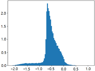
A long tail distribution of the activation values indicates that the activation value is scattered over a large interval, so the variance of the activation values is large. To address the problem of long tail distribution, we use the variance of the activation values as a penalty term to fine tune the ANN model,
where σ is the standard deviation of the activation values. Noting that the standard deviation has the following mathematical properties,
where γ is a constant. Direct optimization of ¯ η = σ2 may not reduce the degree of the long tail phenomenon, since the activation values may be scaled by a constant. We propose to use the following penalty term,
where m is the mean of the activation values, and ϵ is a very small positive number. In the ideal case, if the standard deviation σ is zero after threshold optimization, the value of the activation values becomes a constant 1 after model weight normalization, and only one time step is needed for the converted SNN model.
In some neural networks, the Batch Normalization (BN) layer is in front of the activation function, e.g., the VGG16 model. There are two parameters in the BN layer which represent the standard deviation and mean of the activation values passing through the BN layer. Then the penalty term (23) can be calculated from the parameters of the BN layer.
After fine-tuning the model with the variance penalty (23), trainable clipping layers [Ho and Chang, 2021] are added after the activation functions. The clipping threshold are optimized with L2 regularization,
where θlP and θlN are the positive and negative clipping thresholds in the l-th layer.
4.2 Joint Calibration of Multiple Layers
After threshold optimization, the ANN model can be converted to a SNNmodel. In SNNmodels, the spikes are propagated in both the spatial and temporal domains. But ANN models are trained and fine-tuned in the spatial domain. So the ANN models contain no information about the temporal domain properties of spike sequences. In fact, there are some deviations between the estimated firing rate from ANN and the real firing rate in SNN [Wang et al., 2025]. To compensate for such deviations, the converted SNN models have to be calibrated in the temporal domain.
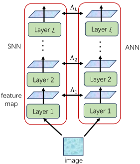
We calibrate the SNN model by using the ANN model as a reference. Neural networks usually consist of multiple layers, each of which output a feature map. In the ideal case, the firing rate of each feature map in the SNN model should be identical to the feature map in the ANN model. Due to the temporal domain properties of spike sequences, there is some deviation between SNN and ANN. We have to fine-tune the SNNmodel such that the deviation is as small as possible.
A conventional method is to calibrate the SNN model layer-by-layer [Wang et al., 2025]. For each layer in the neural network, the input and the output of the layer in the ANN model are saved as a calibration dataset. Then the corresponding layers in the SNN model are fine-tuned with the calibration dataset. Note that the outputs of the shallow layers are the inputs of the deep layers, the calibration errors from the shallow layers are accumulated and grows as the depth of the model goes deeper.
To address the calibration error accumulation problem, we propose to jointly calibrate all layers at the same time. In the proposed joint calibration method, for each layer in the neural network, the loss between the SNN model and the ANN model is calculated, and the averaged loss of all layer is used as the total loss,
where Λl is the loss in the l-th layer, and L is the number of layers.
For the SNNmodel, it is the last layer whose output determines the accuracy of the model. The calibration of the shallow layers should only play an auxiliary role, but every layer in (25) has the same weight. So the model pays too much attention to the shallow layers during training. In particular, when the training is almost finished, the coefficients of the shallow layers are still varying due to the large weight 1/L. So the patterns of the calibration error of the shallow layers are also changing. The deep layers have to keep track of the changes of calibration errors in the shallow layers, which makes it is hard to fine-tune the loss in the last layer.
On the other hand, in the early stage of training, the calibration errors of the shallow layers may vary greatly. In such cases, it is difficult to tune the deep layers since their inputs are from the shallow layers. In other words, we should pay more attention to the shallow layers rather that the deep layers.
As discussed above, in the early stage of multi-layer calibration, we should pay more attention to the shallow layers. As the training processes, the attention should be moved to deep layers. Here we propose a dynamic weighting method, where weights of each layer are adaptive adjusted as the training progresses,
where ϕl(p) is the weight of the l-th layer and p ∈ [0, 1] is the progress of training. The weight of each layer is normalized by dividing ∑l ϕl(p).
When the training progress begins with p = 0, ϕl(p) is a monotonically decreasing function with respect to the layer index l. In this way, the shallow layers are given larger weights while the deep layers are given smaller weights. In other words, we pay more attention to the shallow layers. For the deeper layers in the model, we assigns a small but nonzero positive number, so ϕl(p) > 0, ∀l.
When the training progress ends with p = 1, ϕl(p) is a monotonically increasing function with respect to the layer index l. In this way, the shallow layers are given smaller weights while the deep layers are given larger weights. So more attention is payed on the deep layers in the model.
When the training progress is at the middle stage, 0 < p < 1 , ϕl(p) is a first-increasing and then-decreasing function with respect to the layer index l. The attention is mainly focused on the [pL]-th layer, where [·] is the rounding operation. As the training proceeds, the value of p increases. So the index of the layer with the most attention also increases. In this way, the attention is gradually shifted from the first layer to the last layer.
The weight function ϕl(p) can be designed in several ways. For example, ϕl(p) can be designed based on the cosine function,
ϕl(p) can also be designed based on the sigmoid function,
| Method | ANN | SNN | Time Steps |
|---|---|---|---|
| AugMapping | 92.11% | 92.11% | 220 |
| stReLU | 90.83% | 90.83% | 79 |
| proposed | 92.72% | 92.62% | 10 |
with
5 Experiment Results
5.1 Implementation Details
Variance Penalty. When fine-tuning the model with the variance penalty (23), the total loss function can be written as
where Λc is the original loss function adopted in the training of the ANN model, and λ1 is the weighting factor. The value of η may change dramatically from epoch to epoch during the training. So it is suggested to use an adaptive weighting factor λ1 = 0.1|Λc|/η. The weighting factor λ1 is calculated by detaching from the computation graph of Λc and η.
Surrogate Function. The Heaviside step function is used when the neuron fires spikes in SNN, whose gradient is infinite when the argument of the Heaviside step function is zero. So a surrogate function is needed when training the SNN model in the temporal domain [Wu et al., 2019]. We adopt the sigmoid function as the surrogate function,
where κ is a constant. The sigmoid function g(x) approaches the Heaviside step function as the constant κ increases. In the experiment, κ is set to 6.7, and is increased to 10 after 10 epochs, and is increased to 15 at the 20-th epoch.
Calibration Loss. The calibration loss function is used to measure the difference between the SNN model and the ANN model. In the experiment, we adopt the Kullback-Leibler (KL) Divergence as the calibration loss function,
where P(i) is the activation values in the ANN model, and Q(i) is the firing rate in the SNN model.
5.2 Comparison with State-of-the-art Methods
Table 1 shows the model accuracy of the state-of-the-art algorithms that support negative spikes on the Fashion-MNIST dataset. The network structure under investigation contains two convolutional layers and two linear layers (32c5-p264c5-p2-1024-10), which is the Net4 in [Yu et al., 2022].
| Method | Time Steps | ANN | SNN | ∆acc |
|---|---|---|---|---|
| two-stage | T = 4 | 95.62% | 91.76% | 3.86% |
| proposed | T = 4 | 96.26% | 93.69% | 2.57% |
| two-stage | T = 8 | 95.62% | 93.38% | 2.24% |
| proposed | T = 8 | 96.26% | 95.17% | 1.09% |
| Method | Time Steps | ANN | SNN | ∆acc |
|---|---|---|---|---|
| two-stage | T = 4 | 96.81% | 91.23% | 5.58% |
| proposed | T = 4 | 97.12% | 94.17% | 2.95% |
| two-stage | T = 8 | 96.81% | 93.93% | 2.88% |
| proposed | T = 8 | 97.12% | 95.09% | 2.03% |
The proposed method requires the shortest time step, which is 1/8 of the stReLU method [Han et al., 2023] , and 1/22 of the AugMapping method [Yu et al., 2022]. The AugMapping method is based on the IBT neuron model, so the negative threshold is set to 10 times of the positive threshold. As a result, the neuron has to accumulate within multiple time steps such that the membrane potential exceeds the negative threshold before firing a spike, leading to a very long time step. In the stReLU method, the negative threshold has the same magnitude as the positive threshold, so the firing rate of the negative spikes is on a par with that of the positive spikes. Consequently, the time step of stReLU is shorter than AugMapping. However, the gradient of the stReLU function is zero within two large regions, which leads to a decreased accuracy for the ANN model.
Table 2 shows the model accuracy of VGG-16 on the CIFAR-10 dataset, where ∆acc is the conversion loss in terms of model accuracy. It can be seen that the proposed algorithm suffers from much less accuracy loss than the two-stage algorithm [Wang et al., 2025] under the same time step. For example, when the time step T = 8, the two-stage algorithm suffers an accuracy loss of 2.24%. On the other hand, the proposed algorithm has an accuracy loss of only 1.09%, which is a performance gain of more than 1% compared to the two-stage algorithm. The two-stage algorithm adopts the IBT neuron model, whose negative threshold is too large. Besides, the two-stage algorithm calibrates the converted SNN model in a layer-by-layer fashion. Hence the calibration error are accumulated from shallow layers to deep layers. When the time step T = 4, the proposed algorithm outperforms the two-stage algorithm by 1.29% in terms of accuracy loss. In addition, the accuracy of the proposed algorithm at T = 4 is better than that of the two-stage algorithm at T = 8.
Table 3 shows the model accuracy of ResNet-18 on the CIFAR-10 dataset. Similar results are observed. The proposed algorithm suffers from much less accuracy loss than the two-stage algorithm [Wang et al., 2025] under the same time step, and the accuracy of the proposed algorithm at T = 4 is better than that of the two-stage algorithm at T = 8.
| Threshold Optimization | Layer1 | Layer 2 | Layer 3 |
| with | 0.0964 | 0.0763 | 0.1856 |
|---|---|---|---|
| without | 0.0368 | 0.0161 | 0.0477 |
| Method | ANN | SNN | Time Steps |
|---|---|---|---|
| average cosine sigmoid | 92.72% | 92.61% | 19 |
| 92.72% | 92.62% | 10 | |
| 92.72% | 92.6% | 13 |
5.3 Ablation Study
Now we conduct ablation study on the proposed algorithm. All the ablation experiments are conducted on the FashionMNIST dataset with model Net4. Table 4 shows the firing rate of each layer in Net4. In can be seen that the firing rate is significantly improved with the threshold optimization.
Table 5 shows the performance with different weighting method for the calibration of SNN models in the temporal domain. In can be seen that the averaging method gives the poorest performance since the attention is not adjusted during the training process. For the dynamic weighting method, the weight function based on the cosine function performs slightly better than the one based on the sigmoid function.
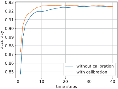
Figure 3 shows the accuracy of the converted SNN model as a function of the time step. It can be seen that if the SNN model is not calibrated in the temporal domain, the accuracy increases slowly after arriving at an accuracy of 92%. About 20 extra time steps are needed to get an accuracy of 92.6%. That is because the ANN model is trained in the spatial domain and contains no information of the spike sequence in the temporal domain. Such mismatch between the temporal domain and the spatial domain can be compensated by extra time steps, as discussed in Section 3. So a longer time step is required for model without calibration.
6 Conclusion
In this paper, we consider the conversion of ANN models to SNN models for the Leaky ReLU function. We design a novel neuron model that supports negative spikes. We show that some neurons may suffer from the long tail distribution problem, and propose a threshold optimization algorithm based on the variance of the activation values. To avoid the problem of error accumulation, we jointly calibrate all layers in the SNN model, where the weight of each layer is adaptive adjusted based on the progress of training.
A Proof of the Membrane Potential Scalar
Let us accumulating (14) from time step 0 to T - 1,
To related (34) to the Leaky ReLU function, let us first consider the case when the input is positive, i.e., f(x) = x, ∀x ⩾ 0. Then only positive spikes are fired, and the firing rate rl ⩾ 0. Eq. (34) becomes
When the time step T is very large, rl can be written as
which align with the positive part of the Leaky ReLU function.
When the input is negative, i.e., f(x) = αx, ∀x < 0. Then only negative spikes are fired, and the firing rate rl < 0. Eq. (34) becomes
When the time step T is very large, β = αN l th /P l th , rl can be written as
which align with the negative part of the Leaky ReLU function.
Acknowledgements
This work was supported in part by National Science and Technology Major Project from Minister of Science and Technology, China (2021ZD0201403), Youth Innovation Promotion Association, Chinese Academy of Sciences (2021233), Shanghai Academic Research Leader (22XD1424500).
@inproceedings{ijcai2025p719,
  title     = {A Fast and Accurate ANN-SNN Conversion Algorithm with Negative Spikes},
  author    = {Wang, Xu and Zhu, Dongchen and Li, Jiamao},
  booktitle = {Proceedings of the Thirty-Fourth International Joint Conference on
               Artificial Intelligence, {IJCAI-25}},
  publisher = {International Joint Conferences on Artificial Intelligence Organization},
  editor    = {James Kwok},
  pages     = {6460--6468},
  year      = {2025},
  month     = {8},
  note      = {Main Track},
  doi       = {10.24963/ijcai.2025/719},
  url       = {https://doi.org/10.24963/ijcai.2025/719},
}
TY - CPAPER TI - A Fast and Accurate ANN-SNN Conversion Algorithm with Negative Spikes AU - Wang, Xu AU - Zhu, Dongchen AU - Li, Jiamao T2 - Proceedings of the Thirty-Fourth International Joint Conference on Artificial Intelligence, IJCAI-25 PB - International Joint Conferences on Artificial Intelligence Organization PY - 2025 SP - 6460 EP - 6468 DO - 10.24963/ijcai.2025/719 UR - https://doi.org/10.24963/ijcai.2025/719 ER -Copied
Machine-readable versions of this paper, for tools and AI agents:





