
Fast Second-Order Online Kernel Learning Through Incremental Matrix Sketching and Decomposition
Proceedings of the Thirty-Fourth International Joint Conference on Artificial Intelligence. Main Track. Pages 6552-6560.
https://doi.org/10.24963/ijcai.2025/729
Keywords
- Machine Learning: ML: Online learning
- Machine Learning: ML: Incremental learning
- Machine Learning: ML: Kernel methods
Abstract
Second-order Online Kernel Learning (OKL) has attracted considerable research interest due to its promising predictive performance in streaming environments. However, existing second-order OKL approaches suffer from at least quadratic time complexity with respect to the pre-set budget, rendering them unsuitable for large-scale datasets. Moreover, the singular value decomposition required to obtain explicit feature mapping is computationally expensive due to the complete decomposition process. To address these issues, we propose FORKS, a fast incremental matrix sketching and decomposition approach tailored for second-order OKL. FORKS constructs an incremental maintenance paradigm for second-order kernelized gradient descent, which includes incremental matrix sketching for kernel approximation and incremental matrix decomposition for explicit feature mapping construction. Theoretical analysis demonstrates that FORKS achieves a logarithmic regret guarantee on par with other second-order approaches while maintaining a linear time complexity w.r.t. the budget, significantly enhancing efficiency over existing methods. We validate the performance of our method through extensive experiments conducted on real-world datasets, demonstrating its superior scalability and robustness against adversarial attacks.
- [Belkin, 2018] Mikhail Belkin. Approximation beats concen- tration? an approximation view on inference with smooth radial kernels. In COLT, volume 75, pages 1348-1361, 2018.
- [Calandriello et al., 2017a] Daniele Calandriello, Alessandro Lazaric, and Michal Valko. Efficient second-order online kernel learning with adaptive embedding. In NIPS, pages 6140-6150, 2017.
- [Calandriello et al., 2017b] Daniele Calandriello, Alessandro Lazaric, and Michal Valko. Second-order kernel online convex optimization with adaptive sketching. In ICML, volume 70, pages 645-653, 2017.
- [CAO et al., 2017] Lele CAO, Fuchun SUN, Hongbo LI, and Wenbing HUANG. Advancing the incremental fusion of robotic sensory features using online multi-kernel extreme learning machine. Frontiers of Computer Science, 11:276, 2017.
- [Cavallanti et al., 2007] Giovanni Cavallanti, Nicolò Cesa- Bianchi, and Claudio Gentile. Tracking the best hyper- plane with a simple budget perceptron. Mach. Learn., 69(2- 3):143-167, 2007.
- [Charikar et al., 2002] Moses Charikar, Kevin C. Chen, and Martin Farach-Colton. Finding frequent items in data streams. In ICALP, volume 2380, pages 693-703, 2002.
- [CHEN et al., 2022] Cheng CHEN, Weinan ZHANG, and Yong YU. Efficient policy evaluation by matrix sketch- ing. Frontiers of Computer Science, 16:165330, 2022.
- [Gao et al., 2022] Chongming Gao, Shijun Li, Wenqiang Lei, Jiawei Chen, Biao Li, Peng Jiang, Xiangnan He, Jiaxin Mao, and Tat-Seng Chua. Kuairec: A fully-observed dataset and insights for evaluating recommender systems. In CIKM, pages 540-550, 2022.
- [Hazan et al., 2007] Elad Hazan, Amit Agarwal, and Satyen Kale. Logarithmic regret algorithms for online convex optimization. Mach. Learn., 69(2-3):169-192, 2007.
- [Hoi et al., 2012] Steven C. H. Hoi, Jialei Wang, Peilin Zhao, Rong Jin, and Pengcheng Wu. Fast bounded online gra- dient descent algorithms for scalable kernel-based online learning. In ICML, 2012.
- [Hu et al., 2015] Junjie Hu, Haiqin Yang, Irwin King, Michael R. Lyu, and Anthony Man-Cho So. Kernelized online imbalanced learning with fixed budgets. In AAAI, pages 2666-2672, 2015.
- [Kane and Nelson, 2014] Daniel M. Kane and Jelani Nel- son. Sparser johnson-lindenstrauss transforms. J. ACM, 61(1):4:1-4:23, 2014.
- [Kivinen et al., 2001] Jyrki Kivinen, Alexander J. Smola, and Robert C. Williamson. Online learning with kernels. In NIPS, pages 785-792, 2001.
- [Liu and Liao, 2015] Yong Liu and Shizhong Liao. Eigenval- ues ratio for kernel selection of kernel methods. In AAAI, pages 2814-2820, 2015.
- [Lu et al., 2016a] Jing Lu, Steven C. H. Hoi, Jialei Wang, Peilin Zhao, and Zhiyong Liu. Large scale online kernel learning. J. Mach. Learn. Res., 17:47:1-47:43, 2016.
- [Lu et al., 2016b] Jing Lu, Peilin Zhao, and Steven C. H. Hoi. Online sparse passive aggressive learning with kernels. In SDM, pages 675-683, 2016.
- [Orabona et al., 2008] Francesco Orabona, Joseph Keshet, and Barbara Caputo. The projectron: a bounded kernel- based perceptron. In ICML, volume 307, pages 720-727, 2008.
- [Sahoo et al., 2019] Doyen Sahoo, Steven C. H. Hoi, and Bin Li. Large scale online multiple kernel regression with application to time-series prediction. ACM Trans. Knowl. Discov. Data, 13(1):9:1-9:33, 2019.
- [Shalev-Shwartz, 2012] Shai Shalev-Shwartz. Online learn- ing and online convex optimization. Found. Trends Mach. Learn., 4(2):107-194, 2012.
- [Singh et al., 2012] Abhishek Singh, Narendra Ahuja, and Pierre Moulin. Online learning with kernels: Overcoming the growing sum problem. In MLSP, pages 1-6, 2012.
- [Wang and Vucetic, 2010] Zhuang Wang and Slobodan Vucetic. Online passive-aggressive algorithms on a budget. In AISTATS, volume 9, pages 908-915, 2010.
- [Wang et al., 2016] Shusen Wang, Luo Luo, and Zhihua Zhang. SPSD matrix approximation vis column selection: Theories, algorithms, and extensions. J. Mach. Learn. Res., 17:49:1-49:49, 2016.
- [Wang et al., 2018] Guanghui Wang, Dakuan Zhao, and Li- jun Zhang. Minimizing adaptive regret with one gradient per iteration. In IJCAI, pages 2762-2768, 2018. IJCAI
- [Williams and Seeger, 2000] Christopher K. I. Williams and Matthias W. Seeger. Using the nyström method to speed up kernel machines. In NIPS, pages 682-688, 2000.
- [Woodruff, 2014] David P. Woodruff. Sketching as a tool for numerical linear algebra. Found. Trends Theor. Comput. Sci., 10(1-2):1-157, 2014.
- [Zhang and Liao, 2018] Xiao Zhang and Shizhong Liao. On- line kernel selection via incremental sketched kernel align- ment. In IJCAI, pages 3118-3124, 2018. IJCAI
- [Zhang and Liao, 2019] Xiao Zhang and Shizhong Liao. In- cremental randomized sketching for online kernel learning. In ICML, volume 97, pages 7394-7403, 2019.
- [Zhang et al., 2023] Xiao Zhang, Ninglu Shao, Zihua Si, Jun Xu, Wenhan Wang, Hanjing Su, and Ji-Rong Wen. Reward imputation with sketching for contextual batched bandits. NIPS, pages 64577-64588, 2023.
- [Zhdanov and Kalnishkan, 2013] Fedor Zhdanov and Yuri Kalnishkan. An identity for kernel ridge regression. Theor. Comput. Sci., 473:157-178, 2013.
- [Zhu and Xu, 2015] Changbo Zhu and Huan Xu. Online gra- dient descent in function space. arXiv, 2015.
- [Zinkevich, 2003] Martin Zinkevich. Online convex program- ming and generalized infinitesimal gradient ascent. In ICML, pages 928-936, 2003.
References were extracted automatically from the PDF and may contain errors.
Full text extracted automatically from the PDF; figures, tables and equations may differ. The PDF is the version of record.
1 Introduction
The objective of online learning is to efficiently and effectively update hypotheses in a data stream environment, where the processes of training and testing are intermixed [ShalevShwartz, 2012]. A popular online learning algorithm is Online Gradient Descent (OGD) [Zinkevich, 2003], which aims to minimize the loss function by iteratively adjusting the parameters in the direction of the negative gradient of the function. To address this limitation, Online Kernel Learning (OKL) maps the input space to a high-dimensional reproducing kernel Hilbert space (RKHS), effectively handling nonlinear learning tasks [Kivinen et al., 2001; Singh et al., 2012;
∗Xiao Zhang and Zhewei Wei are the corresponding authors.
Hu et al., 2015; Lu et al., 2016b; CAO et al., 2017; Sahoo et al., 2019].
From an optimization perspective, OKL can be classified into first-order and second-order methods. First-order methods use a fixed learning rate for gradient descent, resulting in O(√T) regret for any arbitrary sequence of convex losses [Cavallanti et al., 2007; Orabona et al., 2008; Hoi et al., 2012; Lu et al., 2016b; Zhang and Liao, 2019], where T denotes the number of rounds. Although some works set a more aggressive learning rate to improve the regret bound to O(logT), it requires the assumption that the loss function exhibits strong convexity, which is unrealistic for most loss functions [Zhu and Xu, 2015]. In contrast, second-order algorithms utilize the Hessian matrix to adjust the learning rate dynamically, achieving logarithmic regret without requiring strong convexity in all directions [Hazan et al., 2007; Zhdanov and Kalnishkan, 2013; Calandriello et al., 2017a; Calandriello et al., 2017b; Zhang et al., 2023].
Despite the improved regret, exact second-order OKL requires O(t2 ) space and time complexity at round t due to the need to store the entire kernel matrix. Previous studies have primarily focused on approximating the kernel matrix using online sampling techniques [Calandriello et al., 2017a; Calandriello et al., 2017b; CHEN et al., 2022]. However, sampling-based algorithms face two significant issues. First, without prior knowledge of the effective dimension of streaming data, sampling-based methods exhibit at least quadratic time complexity with respect to the budget, which is the maximum size of the static subspace. Second, these methods only address the problem of kernel matrix approximation in online kernel learning and cannot efficiently obtain explicit feature mapping. More precisely, due to the varying size of the subspace, complete singular value decomposition is required to calculate the feature mapping, which is computationally expensive.
In this paper, we propose a fast incremental matrix sketching approach for second-order online kernel learning, along with an efficient decomposition method designed for incremental updates, effectively addressing the two aforementioned challenges both theoretically and experimentally. Our contributions can be summarized as follows:
- We propose FORKS, a fast and effective second-order online kernel learning method that can be generalized to both regression and classification tasks. FORKS
maintains incremental matrix sketching using efficient low-rank modifications and constructs an effective timevarying explicit feature mapping. We provide a detailed theoretical analysis to illustrate the advantages of FORKS, including having linear time complexity w.r.t. the budget, and enjoying a logarithmic regret bound.
- We propose TISVD, a novel incremental singular value decomposition adapting to matrix decomposition problems in online learning environments. We theoretically compare the time complexity between TISVD and the original truncated low-rank SVD, confirming that FORKS with TISVD is computationally more efficient without compromising prediction performance.
- We conduct extensive experiments to demonstrate the superior performance of FORKS on both adversarial and real-world datasets, while also enhancing efficiency. Furthermore, we validate FORKS's robustness and scalability using a large-scale streaming recommendation dataset.
2 Notations and Preliminaries
Let [n] = {1, 2, . . . , n}, upper-case bold letters (e.g., A) represent matrix and lower-case bold letters (e.g., a) represent vectors. We denote by Ai∗ and A∗j the i-th row and j-th column of matrix A, A† the Moore-Penrose pseudoinverse of A, ∥A∥2 and ∥A∥F the spectral and Frobenius norms of A. Let S = {(xt, yt)}Tt=1 ⊆ (X × Y)T be the data stream of T instances, where xt ∈ Rd . We use A = UΣV ⊤ to represent the SVD of A, where U, V denote the left and right matrices of singular vectors and Σ = diag[λ1, ..., λn] is the diagonal matrix of singular values.
2.1 Online Kernel Learning
In this section, we introduce the problem of online kernel learning. Let the kernel function be denoted by κ : X × X → R, with the corresponding kernel matrix K = (κ(xi, xj )), where X represents the input space. Let Hκ denote the reproducing kernel Hilbert space (RKHS) induced by κ, and let the feature mapping ϕ : X → Hκ correspond to this RKHS. In this context, the kernel function can be expressed as the inner product κ(xi, xj ) = ϕ(xi)⊤ϕ(xj ).
Consider a data stream S and a convex loss function ℓ. At round t, we define the hypothesis as ft = w⊤ t ϕ(xt), where xt is the incoming sample. Upon receiving a new example xt, the hypothesis predicts the label ˆ yt using ft. The hypothesis incurs a loss ℓt(ft(xt)) := ℓ(ft(xt), yt), where yt is the true label, and subsequently updates its model parameters. The objective of an online learning algorithm is to bound the cumulative regret, which is defined as:
where f ∗ is the optimal hypothesis, determined in hindsight.
2.2 Matrix Sketching
Given a matrix M ∈ Ra×b , the sketch of M is defined as MS ∈ Ra×s , where S ∈ Rb×s is a sketch matrix. In this paper, we introduce the Sparse Johnson-Lindenstrauss Transform and Column-sampling matrix as the sketch matrix [Charikar et al., 2002; Kane and Nelson, 2014].
Sparse Johnson-Lindenstrauss Transform (SJLT). SJLT is a randomized sketching technique based on hash functions. SJLT consists of D submatrices, written as S = [S1, . . . , SD] ∈ Rb×sp . Each submatrix Sk ∈ Rb×(sp/D) is defined by two sets of hash functions:
where k ∈ {1, . . . ,D}. For each submatrix, the element [Sk]i,j equals gk(i) if j = hk(i), and equals 0 otherwise.
Column-samplingmatrix. We denote the column-sampling matrix by Sm ∈ Rb×sm , the columns of Sm is obtained by uniformly sampling column vectors of Ib×b.
3 FORKS: The Proposed Algorithm
In this section, we propose a novel and efficient second-order OKL method that incorporates incremental sketching and decomposition. While previous work has primarily focused on the incremental maintenance of the approximated kernel matrix, our approach is the first to address the incremental construction and maintenance of the feature mapping.
3.1 AlgorithmOverview
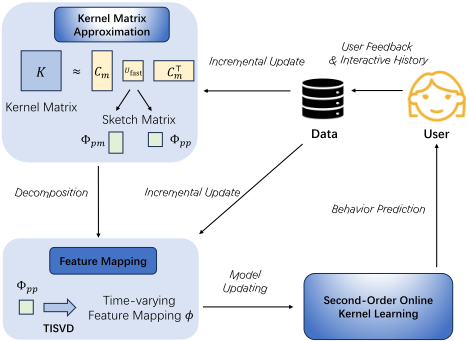
The second-order OKL process can be described in three key stages: kernel matrix approximation, feature mapping, and second-order online learning. Figure 1 illustrates the overall architecture of our method. Rather than storing the entire kernel matrix, we employ matrix sketching techniques to approximate it with a fixed, constant size. Furthermore, the novel truncated incremental singular value decomposition method is utilized to generate the time-varying feature mapping. Notably, both the kernel matrix and feature mapping can be updated incrementally, ensuring efficient maintenance and adaptability to changes in user preferences. Additionally, we use second-order updates to predict user behavior effectively. A non-trivial proof establishes that our method guarantees logarithmic regret while preserving computational efficiency.
3.2 Matrix Sketching for Kernel Matrix Approximation
In this section, we apply the matrix sketching technique to approximate the kernel matrix. Although this reduction has been employed in first-order methods [Zhang and Liao, 2018; Zhang and Liao, 2019], the regret bound for second-order online kernel learning, which operates under the directional curvature condition, remains unknown in the literature.
In the offline setting, given the kernel matrix K(t) ∈ Rt×t , the prototype model [Williams and Seeger, 2000] computes the approximate kernel matrix ˆK(t) = C(t) m Ufast(C(t) m )⊤ by solving the following optimization problem at round t:
where C(t) m represents the sketch matrix at round t, defined as C(t) m = K(t)S(t) m ∈ Rt×sm , with S(t) m ∈ Rt×sm being the column-sampling matrix used to reduce the size of the approximate kernel matrix.
Note that solving Eq. (1) can impose substantial computational demands. To address this problem, the sketch-based method [Wang et al., 2016] is proposed to reduce the computational complexity. Specifically, let S(t) p ∈ Rt×sp represent the randomized sketch matrix based on the SJLT (details in Section 2.2). The sketched kernel matrix approximation problem at round t is then formulated as follows:
where
Instead of storing the entire kernel matrix, we can maintain smaller sketches for approximation. In the online setting, these sketches can be incrementally updated with the arrival of new data, xt+1. Specifically, the updates are given by:
where ∆(t+1) pm and∆(t+1) pp are composed of three rank-1 matrices. Due to space constraints, the detailed construction is provided in Appendix B.1.
Next, we construct the time-varying explicit feature mapping. For simplicity, we use rank-k SVD, though it is inefficient due to the need for a full matrix decomposition. The elements of the kernel matrix are equal to the inner product of the corresponding points after feature mapping, i.e.
Ki,j = ϕ(xi)⊤ϕ(xj). Once we build the approximate kernel matrix by Eq. (2), we can obtain a time-varying feature mapping through the rank-k SVD. Specifically, if
where V (t+1) ∈ Rsp×k , Σ(t+1) ∈ Rk×k and rank k ≤ sp, we can update the time-varying explicit feature mapping ϕt+2 ∈ Rk at round t + 1 by
where {˜xi}sm i=1 are the sampled columns by S(t+1) m and Zt+1 = (Φ(t+1) pm )†V (t+1) (Σ(t+1) ) 12 .
However, directly applying rank-k SVD to Φpp is inefficient in online learning scenarios. Specifically, the standard rankk SVD incurs a time complexity of O(s3p ) at each update, rendering it impractical in scenarios with frequent updates.
3.3 Novel Incremental Matrix Decomposition Method for Feature Mapping
In this section, we propose TISVD (Truncated Incremental Singular Value Decomposition), a novel incremental SVD method designed for decomposing sketches. TISVD achieves linear time and space complexity with respect to the sketch size sp, effectively avoiding the time-consuming operation of performing a complete SVD.
We begin by presenting the construction of TISVD, which is well-suited for decomposing matrices with low-rank update properties. Without loss of generality, we denote a matrix at round t as M (t) = U (t)Σ(t)V (t)⊤. In the (t + 1)-th round, M (t) is updated by low-rank matrices as follows:
where ∆1,∆2 ∈ Rsp×c of rank r ≤ c ≪ sp.
Our objective is to directly update the singular matrices U (t) , Σ(t) and V (t) using low-rank update matrices ∆1 and ∆2, resulting in U (t+1) , Σ(t+1) and V (t+1) . First, we formulate orthogonal matrices through orthogonal projection and vertical projection. Let P , Q denote the orthogonal basis of the column space of the following matrices:
where
Subsequently, as the size of H is smaller thanM(t+1) , an efficient computation of ˜Uk, ˜ Vk, and ˜Σk can be obtained by performing a truncated rank-k SVD on H. Since the matrices on the left and right sides are column orthogonal, we finally obtain U (t+1) , V (t+1) , and Σ(t+1) at round t + 1:
We summarize the algorithm and provide the pseudo-code for TISVD in Appendix B.2. Note that the sketch Φ(t+1) pp can be updated using low-rank matrices, as shown in Eq. (4). By replacing the standard rank-k SVD with TISVD, we establish an efficient mechanism for the incremental maintenance of singular matrices. More precisely, in Eq. (5), we update V (t+1) and Σ(t+1) using their previous counterparts, V (t) and Σ(t) , along with the low-rank update ∆(t+1) pp at round t +1.
Remark 1 (Complexity). The complexity of TISVD is primarily composed of the truncated rank-k SVD on H and the matrix multiplication in Eq. (9). The update cost of the truncated rank-k SVD is O(k3 ), while the matrix multiplication in Eq. (9) incurs a complexity of O(spk). Consequently, compared to standard rank-k SVD, TISVD provides significant improvements by reducing the time complexity from O(s3p ) to O(spk + k3 ) and the space complexity from O(s2p ) to O(spk + k2 ). More discussion is provided in Appendix B.3.
3.4 Efficient Second-Order Online Kernel Learning
Since the efficient time-varying explicit feature mapping ϕt(·) has been constructed, we can formulate the approximate hypothesis ft(xt) at round t as follows
where wt is the weight vector. On the basis of the hypothesis, we propose a two-stage second-order online kernel learning method, named FORKS (Fast Second-Order Online Kernel Learning Using Incremental Sketching).
In the first stage, we simply collect the items with nonzero losses to the buffer SV and perform the Kernelized Online Gradient Descent (KOGD) [Kivinen et al., 2001]. When the size of the buffer reaches a fixed budget B, we calculate Kt and initialize sketch matrices Φ(t) pp , Φ(t) pm in Eq. (3).
In the second stage, we adopt a periodic updating strategy for sketches. More precisely, we update Φ(t) pp , Φ(t) pm by Eq. (4) once for every ρ examples, where ρ ∈ [T - B] is defined as update cycle. Furthermore, we incrementally update the feature mapping ϕt(·) by TISVD.
In addition to updating the feature mapping ϕt(·), we perform second-order updates on the wt. Specifically, we update the hypothesis using Online Newton Step (ONS) [Hazan et al., 2007] for some parameters α > 0 and σi, ηi ≥ 0:
where gt = ∇wt ℓt(ˆ yt), At = αI + ∑ti=0 (σi + ηi)gig⊤ i and h(z) = sign(z)max(|z| - C, 0). The second-order updates
Algorithm 1 FORKS
Input: Data stream {(xt, yt)}Tt=1 , sketch size sp, sample size sm, rank k, budget B, update cycle ρ, regularizer α Output: Predicted label {ˆ yt}Tt=1
- 1: for t ← 1, . . . , T do
- 2: Receive xt
- 3: while SV is not full do
- 4: Update hypothesis by KOGD
- 5: Add xt to SVwhenever the loss is nonzero
- 6: end while
- 7: if SV is full then 8: Initialize Φ(t) pp , Φ(t) pm as in Eq. (3)
9: Compute the mapping ϕt+1
- 10: else if in the update round then
11: Update ϕt+1 by TISVD (Algorithm 2)
- 12: Set At ←αI, wt ← 0
- 13: else
- 15: end if
- 16: Predict ˆ yt = sgn (ϕ⊤t wt )
- 17: # Execute a second-order gradient descent
- 18: Obtain gt ←∇wt ℓt (ˆ yt)
- 19: Update At+1 ←At + (σi + ηi)gtg⊤ t
- 20: Compute wt+1, vt+1 using Eq. (10)
- 21: end for
not only consider the gradient information but also utilize the curvature information of the loss function, leading to faster convergence rates.
At the start of a new update epoch, we incorporate a reset step before applying the gradient descent in the new embedded space. We update the feature mapping ϕt but reset At and wt. This step is taken to ensure that our starting point cannot be influenced by the adversary. By leveraging efficient second-order updates, we can effectively converge to the optimal hypothesis within the current subspace. Furthermore, the reset of the descent procedure when transitioning between subspaces ensures a stable starting point and maintains a bounded regret throughout the entire process. We summarize the above stages into Algorithm 1.
The incremental update of the feature mapping, combined with the reset mechanism, ensures that we can effectively capture changes in user preferences over time. More specifically, our algorithm updates the feature vector to reflect the user's current state, while resetting the Hessian matrix mitigates the influence of outdated data on the learner.
3.5 Complexity Analysis of FORKS
Given the budget of B, FORKS consists of three parts: (1) the first stage using KOGD, (2) the updating round in the second stage, and (3) the regular round in the second stage. At the first stage (|SV | ≤ B), FORKS has constant time O(B) and space complexities O(B) per round.
The main computational complexity of FORKS during the update round stems from the matrix decomposition and inversion procedures. These processes are necessary for updating the feature mapping and performing second-order updates, respectively. TISVD reduces the time complexity of Φpp decomposition from O(s3p ) to O(spk + k3 ), where sp is the sketch size of Sp and k is the rank in TISVD. A naive implementation of the second-order update requires O(k3 ) per-step time and has a space complexity of O(k2 ) necessary to store the Hessian At. By taking advantage of the fact that At is rank-1 updated, we can reduce the per-step cost to O(k2 ).
We denote the update cycle as ρ and µ = B+⌊(T - B)/ρ⌋. To summarize, the time complexity of FORKS at each updating round is
and the space complexity is O(µ + spk + smsp + k2 ), where sm is the sketch size of Sm.
The primary time consumption for the online learning algorithm occurs during regular rounds. At each regular round, the time complexity of FORKS is O(smk + k2 ). Given that sm < sp < B, our algorithm achieves a time complexity of O(Bk+k2 ) per step. The current state-of-the-art second-order online kernel learning method, PROS-N-KONS, presents a time complexity of O(B2 ) per step in its budget version [Calandriello et al., 2017a]. Moreover, due to the changing size of the subspace from online sampling, PROS-N-KONS must perform a complete SVD at each step. In contrast, FORKS introduces substantial advancements by reducing the time complexity from O(B2 ) to O(Bk + k2 ).
4 Regret Analysis
In this section, we provide the regret analysis for the proposed second-order online kernel learning algorithm. We begin by making the following assumptions about the loss functions.
Assumption 1 (Lipschitz Continuity). ℓ is Lipschitz continuous with the Lipschitz constant LLip, i.e., ∥∇ℓ(w)∥2 ≤ LLip.
Assumption 2 (Directional Curvature). Let LCur ≥ 0. Then, for any vectors w1,w2 and the convex function ℓ, denote that ∆ = ℓ(w1) - ℓ(w2), we have
In practical scenarios, the assumption of strong convexity may not always hold as it imposes constraints on the convexity of losses in all directions. Amore feasible approach is to relax this assumption by demanding strong convexity only in the gradient direction, which is a weaker condition as indicated by the two assumptions above. For example, exp-concave losses like squared loss and squared hinge loss satisfy Assumption 2.
Assumption 3 (Matrix Product Preserving). Let Sp ∈ RT×sp be a sketch matrix, Um ∈ RT×sm be a matrix with orthonormal columns, U ⊥ m ∈ RT×(T-sm) be another matrix satisfying UmU ⊤ m +U ⊥ m (U ⊥ m )⊤ = IT and U ⊤ m U ⊥ m = O, and δi (i = 1, 2) be the failure probabilities defined as follows:
where A1 = Um, B1 = IT , A2 = U ⊥ m (Um⊥)⊤K, B2 = U ⊤ m , K ∈ RT×T is a kernel matrix.
The conditions stated in Assumption 3 can be satisfied by SJLT matrix [Woodruff, 2014]. Given the loss ℓt(wt) := ℓt(ft) = ℓ(ft(xt), yt), ∀t ∈ [T] satisfies Assumption 1 and Assumption 2, we bound the following regret:
where f ∗ = argminf∈Hκ ∑Tt=1 ℓt(f) denotes the optimal hypothesis in hindsight in the original RKHS.
Let K ∈ RT×T be a kernel matrix with κ(xi, xj) ≤ 1 for all i, j. Let ρ = ⌊θ(T -B)⌋ denote the update cycle, where θ ∈ (0, 1), and let k represent the rank in TISVD. Additionally, define CCoh as the coherence of the intersection matrix of K, which is constructed using B + ⌊(T - B)/ρ⌋ examples. Let vi be the i-th singular vector of K, the coherence is given by:
Note that CCoh is independent of T when ρ = ⌊θ(T -B)⌋. We demonstrate the regret upper bound of FORKS as follows
Theorem 1 (Regret Bound of FORKS). Let δ0, ϵ0 ∈ (0, 1). Set the number of submatrices in SJLT as D = Θ(log3 (sm)). Suppose the parameters for updating At in FORKS satisfy ηi = 0 and σi ≥ LCur > 0. Assume the eigenvalues of K decay polynomially with decay rate β > 1, and that the SJLT Sp satisfies Assumption 3 with failure probabilities δ1, δ2 ∈ (0, 1). If the sketch sizes of Sp and Sm satisfy
Then, with probability at least 1 - δ,
where δ = δ0+δ1+δ2, Dw denotes the diameter of the weight vector space of the hypothesis on the incremental sketches, and ϵ is defined as:
proof sketch. Let w∗ denote the optimal hypothesis on the incremental sketches in hindsight, we decompose the instantaneous regret ℓt(wt) - ℓt(w∗ ) into two terms as follows
The optimization error stems from the optimization step of second-order online gradient descent, while the estimation error arises from the incremental matrix sketching and the truncated singular values in TISVD. We provide upper bounds for the errors and present the detailed proof in Appendix C.1.
Remark 2 (Assumption of polynomial decay). The assumption of polynomial eigenvalue decay for the kernel matrix is widely applicable and holds for various types of kernels, including shift-invariant, finite-rank, and convolution kernels [Liu and Liao, 2015; Belkin, 2018]. This decay property guarantees that the accumulated truncated singular values of TISVD can be upper bounded by the number of update rounds.
Remark 3 (Convex case). Note that when LCur = 0, Assump-
tion 2 essentially enforces convexity. In the worst case when LCur = 0, the regret bound in the convex case degenerates to O(√T). The detailed proof is included in Appendix C.2.
By configuring the update cycle as ρ = ⌊θ(T - B)⌋, where θ ∈ (0, 1), and setting the sketch size ratio to γ = O(log(T)/√T), we derive an upper bound on regret of O(T 14 logT) for second-order online kernel learning. In contrast, the regret bound for first-order online kernel learning is O(√T ), while requiring a budget of B = O(T ) [Lu et al., 2016a], making it less favorable than FORKS.
Under the assumption that the eigenvalues of the kernel matrix decay polynomially with rate β, the regret bound for the existing second-order online kernel learning algorithm PROS-N-KONS [Calandriello et al., 2017a] is O(T 1β log2 T), which is highly sensitive to the eigenvalue decay rate β. In practical streaming scenarios, however, ensuring a sufficiently rapid decay of the kernel matrix is often unrealistic. When the properties of the streaming matrix are less favorable, such as in the case where β < 4, the regret of PROS-N-KONS can be worse than that of FORKS.
5 Experiments
In this section, we conduct experiments to evaluate the performance of FORKS on several datasets. The details of datasets and experimental setup are presented in Appendix D.1, D.2.
5.1 Experiments Under a Fixed Budget
In this section, we demonstrate the performance of FORKS under a fixed budget, employing six widely recognized classification benchmarks. We compare FORKS with the existing budgeted-based online learning algorithms, including first-order algorithms RBP [Cavallanti et al., 2007], BPAS [Wang and Vucetic, 2010], BOGD [Hoi et al., 2012], FOGD, NOGD [Lu et al., 2016a], Projectron [Orabona et al., 2008], SkeGD [Zhang and Liao, 2019] and second-order algorithm PROS-N-KONS [Calandriello et al., 2017a]. All algorithms are trained using hinge loss, and their performance is measured by the average online mistake rate.
For all the algorithms, we set a fixed budget B = 50 for small datasets (N ≤ 10000) and B = 100 for large datasets. Furthermore, we set buffer size ˜B = 2B, γ = 0.2, sp = B, sm = γsp, θ = 0.3, and update cycle ρ = ⌊θN⌋ in SkeGD and FORKS if not specially specified. For algorithms with rank-k approximation, we uniformly set k = 0.1B. Besides, we use the same experimental settings for FOGD (feature dimension = 4B). The results are presented in Table 1. Our FORKS shows the best performance on svmguide3, codrna, w7a, and the suboptimal performance on other datasets. The update time of FORKS is comparable to that of the majority of first-order algorithms, including NOGD and SkeGD. Besides, FORKS is significantly more efficient than the existing second-order method PROS-N-KONS in largescale datasets such as codrna and w7a.
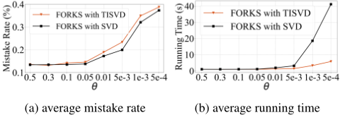
Then, we conduct experiments to evaluate how TISVD affects the performance of the algorithm. We use the same experimental setup in codrna and vary the update rate θ from 0.5 to 0.0005. Figure 2 demonstrates that TISVD maintains efficient decomposition speed without excessively reducing performance. Considering that frequent updates can potentially result in an elevated loss, it is essential to carefully choose an optimal update cycle that strikes a balance between achieving superior accuracy and maintaining efficiency.
5.2 Experiments Under Adversarial Environment
To empirically validate the algorithms under an adversarial environment, we build adversarial datasets using the benchmark codrna and german. We compare FORKS with firstorder algorithms BOGD [Hoi et al., 2012], SkeGD [Zhang and Liao, 2019], NOGD [Lu et al., 2016a] and second-order algorithm PROS-N-KONS [Calandriello et al., 2017a] under the same budget B = 200. Besides, we set γ = 0.2, sp = 0.75B, sm = γsp, k = 0.1B and update cycle ρ = ⌊0.005(N-B)⌋ in SkeGD and FORKS. Inspired by the adversarial settings in [Calandriello et al., 2017a; Wang et al., 2018; Zhang and Liao, 2019], we generate an online learning game with b blocks. At each block, we extract an instance from the dataset and repeat it for r rounds. In addition, the labels are flipped in each even block by multiplying them with -1. We set b = 500, r = 10 for codrna-1 and german-1.
Experimental results are presented in Table 2. It is observed that in the adversarial environment, the performance of all methods significantly decreases with the increase of adversarial changes except for FORKS. This is due to the fact that FORKS accurately captures the concept drifting through the incremental update of the sketch matrix and the execution of rapid second-order gradient descent. Moreover, FORKS maintains its efficiency comparable to first-order algorithms, thereby ensuring that improved performance is achieved without sacrificing computational time.
5.3 Experiments on Large-Scale Datasets
In this experiment, we evaluate the efficiency and effectiveness of FORKS on streaming recommendation. We use KuaiRec, which is a real-world dataset collected from the recommendation logs of the video-sharing mobile app Kuaishou [Gao et al., 2022]. We conduct experiments on the dense matrix of KuaiRec, which consists of 4, 494, 578 instances with associated timestamps, making it an ideal benchmark for evaluating large-scale online learning tasks. We test the performance of the algorithm used in Section 5.3 under different budgets B ranging from 100 to 500. To avoid excessive training time, we use a budgeted version of PROS-N-KONS that stops updating the dictionary at a maximum budget of Bmax = 100. Since the buffer size of PROS-N-KONS is data-dependent, we repeat the training process 20 times to compute the average error rate and the average time for comparison. In addition to the hinge loss, we use squared hinge loss to evaluate the performance.
| Algorithm | german | svmguide3 | spambase | |||
|---|---|---|---|---|---|---|
| Mistake rate | Time | Mistake rate | Time | Mistake rate | Time | |
| RBP | 38.830 ± 0.152 | 0.003 | 29.698 ± 1.644 | 0.003 | 35.461 ± 0.842 | 0.025 |
| BPA-S | 35.235 ± 0.944 | 0.004 | 29.027 ± 0.732 | 0.004 | 34.394 ± 2.545 | 0.039 |
| Projectron | 36.875 ± 1.403 | 0.003 | 25.060 ± 0.373 | 0.003 | 32.659 ± 0.914 | 0.031 |
| BOGD | 33.705 ± 1.446 | 0.007 | 29.904 ± 1.653 | 0.006 | 32.859 ± 0.478 | 0.049 |
| FOGD | 30.915 ± 0.845 | 0.025 | 30.024 ± 0.787 | 0.022 | 25.651 ± 0.349 | 0.175 |
| NOGD | 26.715 ± 0.552 | 0.014 | 19.964 ± 0.077 | 0.008 | 31.003 ± 0.751 | 0.077 |
| SkeGD | 25.170 ± 0.391 | 0.009 | 19.976 ± 0.105 | 0.007 | 32.413 ± 1.886 | 0.067 |
| PROS-N-KONS | 31.235 ± 0.939 | 1.017 | 24.529 ± 0.561 | 0.015 | 32.227 ± 0.678 | 6.638 |
| FORKS (Ours) | 26.425 ± 0.562 | 0.008 | 19.710 ± 0.557 | 0.009 | 30.662 ± 0.670 | 0.070 |
| Algorithm | codrna | w7a | ijcnn1 | |||
| Mistake rate | Time | Mistake rate | Time | Mistake rate | Time | |
| RBP | 22.644 ± 0.262 | 0.210 | 5.963 ± 0.722 | 0.945 | 21.024 ± 0.578 | 0.633 |
| BPA-S | 17.029 ± 0.303 | 0.313 | 3.001 ± 0.045 | 1.145 | 11.114 ± 0.064 | 0.747 |
| Projectron | 19.257 ± 4.688 | 0.341 | 3.174 ± 0.014 | 0.965 | 9.478 ± 0.001 | 0.621 |
| BOGD | 17.305 ± 0.146 | 0.507 | 3.548 ± 0.164 | 0.970 | 11.559 ± 0.174 | 0.724 |
| FOGD | 13.103 ± 0.105 | 1.480 | 2.893 ± 0.053 | 2.548 | 9.674 ± 0.105 | 3.125 |
| NOGD | 17.915 ± 3.315 | 0.869 | 2.579 ± 0.007 | 2.004 | 9.379 ± 0.001 | 1.457 |
| SkeGD | 13.274 ± 0.262 | 0.779 | 2.706 ± 0.335 | 2.093 | 11.898 ± 1.440 | 2.216 |
| PROS-N-KONS | 13.387 ± 0.289 | 114.983 | 3.016 ± 0.007 | 92.377 | 9.455 ± 0.001 | 5.000 |
| FORKS (Ours) | 12.795 ± 0.360 | 0.918 | 2.561 ± 0.038 | 2.240 | 9.381 ± 0.001 | 2.480 |
| Algorithm | codrna-1 | german-1 | ||
|---|---|---|---|---|
| Mistake rate | Time | Mistake rate | Time | |
| BOGD | 26.066 ± 1.435 | 0.029 | 32.131 ± 1.079 | 0.042 |
| NOGD | 29.780 ± 1.257 | 0.024 | 28.103 ± 1.247 | 0.040 |
| SkeGD | 24.649 ± 5.087 | 0.269 | 11.026 ± 4.018 | 0.113 |
| PROS-N-KONS | 21.299 ± 1.364 | 3.323 | 17.174 ± 1.437 | 0.477 |
| FORKS (Ours) | 6.752 ± 1.647 | 0.023 | 5.142 ± 0.215 | 0.035 |
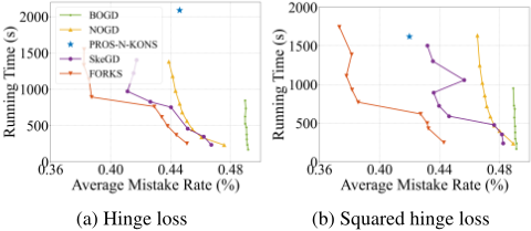
Figure 3 (a) shows the tradeoff between running time and the average mistake rate in the experiment using hinge loss. Figure 3 (b) shows the tradeoff between running time and the average mistake rate in the experiment using squared hinge loss. We observe that FORKS consistently achieves superior learning performance while maintaining comparable time costs to the other first-order algorithms, regardless of the loss function's shape. In particular, for squared hinge loss, both PROS-N-KONS and FORKS significantly outperform firstorder models, highlighting the advantages of second-order methods under exp-concave losses. We also observe that FORKS demonstrates considerably higher efficiency than the second-order algorithm PROS-N-KONS. Under squared hinge loss, to achieve a comparable online error rate, FORKS requires only approximately 500 seconds, while PROS-N-KONS takes over 1500 seconds, resulting in a threefold speedup.
6 Conclusion
This paper introduces FORKS, a fast second-order online kernel learning approach. By leveraging incremental matrix sketching and decomposition techniques, FORKS efficiently addresses the computational challenges inherent in kernel feature mapping and hypothesis updates. The proposed method achieves a logarithmic regret bound while maintaining linear time complexity relative to the budget, significantly improving the efficiency of existing second-order methods. Extensive experimental evaluations on various datasets demonstrate the superior scalability and robustness of our approach.
Acknowledgments
This research was supported in part by National Science and Technology Major Project (2022ZD0114802), by National Natural Science Foundation of China (No. 92470128, No. U2241212, No. 62376275), by Beijing Outstanding Young Scientist Program No.BJJWZYJH012019100020098, by Huawei-Renmin University joint program on Information Retrieval. We also wish to acknowledge the support provided by the fund for building world-class universities (disciplines) of Renmin University of China, by Engineering Research Center of Next-Generation Intelligent Search and Recommendation, Ministry of Education, by Intelligent Social Governance Interdisciplinary Platform, Major Innovation & Planning Interdisciplinary Platform for the "Double-First Class" Initiative, Public Policy and Decision-making Research Lab, and Public Computing Cloud, Renmin University of China. The work was partially done at Beijing Key Laboratory of Research on Large Models and Intelligent Governance, MOE Key Lab of Data Engineering and Knowledge Engineering, Engineering Research Center of Next-Generation Intelligent Search and Recommendation, MOE, and Pazhou Laboratory (Huangpu), Guangzhou, Guangdong 510555, China.
@inproceedings{ijcai2025p729,
  title     = {Fast Second-Order Online Kernel Learning Through Incremental Matrix Sketching and Decomposition},
  author    = {Wen, Dongxie and Zhang, Xiao and Wei, Zhewei and Hou, Chenping and Li, Shuai and Zhang, Weinan},
  booktitle = {Proceedings of the Thirty-Fourth International Joint Conference on
               Artificial Intelligence, {IJCAI-25}},
  publisher = {International Joint Conferences on Artificial Intelligence Organization},
  editor    = {James Kwok},
  pages     = {6552--6560},
  year      = {2025},
  month     = {8},
  note      = {Main Track},
  doi       = {10.24963/ijcai.2025/729},
  url       = {https://doi.org/10.24963/ijcai.2025/729},
}
TY - CPAPER TI - Fast Second-Order Online Kernel Learning Through Incremental Matrix Sketching and Decomposition AU - Wen, Dongxie AU - Zhang, Xiao AU - Wei, Zhewei AU - Hou, Chenping AU - Li, Shuai AU - Zhang, Weinan T2 - Proceedings of the Thirty-Fourth International Joint Conference on Artificial Intelligence, IJCAI-25 PB - International Joint Conferences on Artificial Intelligence Organization PY - 2025 SP - 6552 EP - 6560 DO - 10.24963/ijcai.2025/729 UR - https://doi.org/10.24963/ijcai.2025/729 ER -Copied
Machine-readable versions of this paper, for tools and AI agents:





