
General Incomplete Time Series Analysis via Patch Dropping Without Imputation
Proceedings of the Thirty-Fourth International Joint Conference on Artificial Intelligence. Main Track. Pages 6597-6605.
https://doi.org/10.24963/ijcai.2025/734
Keywords
- Machine Learning: ML: Time series and data streams
Abstract
Missing values in multivariate time series data present significant challenges to effective analysis. Existing methods for multivariate time series analysis either ignore missing data, sacrificing performance, or follow the impute-then-analyze paradigm, which suffers from redundant training and error accumulation, leading to biased results and suboptimal performance. In this paper, we propose INTER, a novel end-to-end framework for incomplete multivariate time series analysis, which bypasses imputation by leveraging pre-trained language models to learn the distribution of incomplete time series data. INTER incorporates two novel components: the missing-rate-aware time series patch-dropping (MPD) strategy and the missing-aware Transformer block, both of which we propose to enhance model generalization, robustness, and the ability to capture underlying patterns in the observed incomplete time series. Moreover, we theoretically prove that the MPD strategy exhibits lower sample variance for time series with the same dropout rate compared to other dropping strategies. Extensive experiments on 11 public real-world time series datasets demonstrate that INTER improves accuracy by over 20% compared to state-of-the-art methods, while maintaining competitive computational efficiency.
- [Bagnall et al., 2018] Anthony Bagnall, Hoang Anh Dau, Ja- son Lines, Michael Flynn, James Large, Aaron Bostrom, Paul Southam, and Eamonn Keogh. The uea multivari- ate time series classification archive, 2018. arXiv preprint arXiv:1811.00075, 2018.
- [Bartholomew, 1971] David J Bartholomew. Time series analysis forecasting and control. Journal of the Opera- tional Research Society, 22(2):199-201, 1971.
- [Buuren and Groothuis-Oudshoorn, 2010] S van Buuren and Karin Groothuis-Oudshoorn. mice: Multivariate imputa- tion by chained equations in r. Journal of Statistical Soft- ware, pages 1-68, 2010.
- [Cao et al., 2018] Wei Cao, Dong Wang, Jian Li, Hao Zhou, Lei Li, and Yitan Li. Brits: Bidirectional recurrent imputa- tion for time series. In NeurIPS, pages 6775-6785, 2018.
- [Che et al., 2018] Zhengping Che, Sanjay Purushotham, Kyunghyun Cho, David Sontag, and Yan Liu. Recurrent neural networks for multivariate time series with missing values. Scientific Reports, 8(1):6085, 2018.
- [Coletta et al., 2024] Andrea Coletta, Sriram Gopalakrish- nan, Daniel Borrajo, and Svitlana Vyetrenko. On the con- strained time-series generation problem. Advances in Neu- ral Information Processing Systems, 36, 2024.
- [Du et al., 2023] Wenjie Du, David Côté, and Yan Liu. Saits: Self-attention-based imputation for time series. Expert Systems with Applications, 219:119619, 2023.
- [Ekambaram et al., 2023] Vijay Ekambaram, Arindam Jati, Nam Nguyen, Phanwadee Sinthong, and Jayant Kalagnanam. Tsmixer: Lightweight mlp-mixer model for multivariate time series forecasting. In Proceedings of the 29th ACM SIGKDD Conference on Knowledge Discovery and Data Mining, pages 459-469, 2023.
- [Feng et al., 2023] Raymond Feng, Flavio P Calmon, and Hao Wang. Adapting fairness interventions to missing val- ues. In NeurIPS, pages 59388-59409, 2023.
- [Feng et al., 2024] Yu Feng, Zhen Tian, Yifan Zhu, Zongfu Han, Haoran Luo, Guangwei Zhang, and Meina Song. Cp- prompt: Composition-based cross-modal prompting for domain-incremental continual learning. In Proceedings of the 32nd ACM International Conference on Multimedia, pages 2729-2738, 2024.
- [Feng et al., 2025] Yu Feng, Yangli-ao Geng, Yifan Zhu, Zongfu Han, Xie Yu, Kaiwen Xue, Haoran Luo, Mengyang Sun, Guangwei Zhang, and Meina Song. Pm- moe: Mixture of experts on private model parameters for personalized federated learning. In Proceedings of the ACM on Web Conference 2025, pages 134-146, 2025.
- [Franceschi et al., 2019] Jean-Yves Franceschi, Aymeric Dieuleveut, and Martin Jaggi. Unsupervised scalable representation learning for multivariate time series. In NeurIPS, volume 32, pages 1-12, 2019.
- [Gasparin et al., 2022] Alberto Gasparin, Slobodan Lukovic, and Cesare Alippi. Deep learning for time series forecast- ing: The electric load case. CAAI Transactions on Intelli- gence Technology, 7(1):1-25, 2022.
- [Goel et al., 2022] Karan Goel, Albert Gu, Chris Donahue, and Christopher Ré. It's raw! audio generation with state- space models. In ICML, pages 7616-7633, 2022.
- [Goldberger et al., 2000] Ary L Goldberger, Luis AN Ama- ral, Leon Glass, Jeffrey M Hausdorff, Plamen Ch Ivanov, Roger G Mark, Joseph E Mietus, George B Moody, Chung-Kang Peng, and H Eugene Stanley. Physiobank, physiotoolkit, and physionet: components of a new re- search resource for complex physiologic signals. circu- lation, 101(23):e215-e220, 2000.
- [Kraskov et al., 2004] Alexander Kraskov, Harald Stögbauer, and Peter Grassberger. Estimating mutual information. Physical Review E-Statistical, Nonlinear, and Soft Matter Physics, 69(6):066138, 2004.
- [Li et al., 2022] Yan Li, Xinjiang Lu, Yaqing Wang, and De- jing Dou. Generative time series forecasting with diffu- sion, denoise, and disentanglement. Advances in Neural Information Processing Systems, 35:23009-23022, 2022.
- [Liang et al., 2024] Yuxuan Liang, Haomin Wen, Yuqi Nie, Yushan Jiang, Ming Jin, Dongjin Song, Shirui Pan, and Qingsong Wen. Foundation models for time series anal- ysis: A tutorial and survey. In Proceedings of the 30th ACM SIGKDD conference on knowledge discovery and data mining, pages 6555-6565, 2024.
- [Liao et al., 2024] Weibin Liao, Yifan Zhu, Yanyan Li, Qi Zhang, Zhonghong Ou, and Xuesong Li. Revgnn: Negative sampling enhanced contrastive graph learning for academic reviewer recommendation. ACM Transactions on Information Systems, 43(1):1-26, 2024.
- [Lim and Zohren, 2021] Bryan Lim and Stefan Zohren. Time-series forecasting with deep learning: a sur- vey. Philosophical Transactions of the Royal Society A, 379(2194):20200209, 2021.
- [Liu et al., 2024] Yong Liu, Haoran Zhang, Chenyu Li, Xi- angdong Huang, Jianmin Wang, and Mingsheng Long. Timer: Generative pre-trained transformers are large time series models. In ICML, 2024.
- [Makridakis, 2018] Spyros Makridakis. M4 dataset, 2018. https://github.com/M4Competition/M4-methods/ tree/master/Dataset (Accessed: 2025-01-24). Link
- [Miao et al., 2021] Xiaoye Miao, Yangyang Wu, Jun Wang, Yunjun Gao, Xudong Mao, and Jianwei Yin. Generative semi-supervised learning for multivariate time series im- putation. In AAAI, pages 8983-8991, 2021.
- [Miao et al., 2022] Xiaoye Miao, Yangyang Wu, Lu Chen, Yunjun Gao, Jun Wang, and Jianwei Yin. Efficient and effective data imputation with influence functions. Pro- ceedings of the VLDB Endowment, 15(3):624-632, 2022.
- [Moody et al., 2011] George B Moody, Roger G Mark, and Ary L Goldberger. Physionet: Physiologic signals, time series and related open source software for basic, clinical, and applied research. In 2011 Annual International Con- ference of the IEEE Engineering in Medicine and Biology Society, pages 8327-8330. IEEE, 2011.
- [Nie et al., 2022] Yuqi Nie, Nam H Nguyen, Phanwadee Sinthong, and Jayant Kalagnanam. A time series is worth 64 words: Long-term forecasting with transformers. In ICLR, pages 1-24, 2022.
- [Radford et al., 2019] Alec Radford, Jeffrey Wu, Rewon Child, David Luan, Dario Amodei, Ilya Sutskever, et al. Language models are unsupervised multitask learners. OpenAI Blog, 1(8):9, 2019.
- [Silva et al., 2012] Ikaro Silva, George Moody, Daniel J Scott, Leo A Celi, and Roger G Mark. Predict- ing in-hospital mortality of icu patients: The phys- ionet/computing in cardiology challenge 2012. In CINC, pages 245-248, 2012.
- [Tashiro et al., 2021] Yusuke Tashiro, Jiaming Song, Yang Song, and Stefano Ermon. Csdi: Conditional score-based diffusion models for probabilistic time series imputation. In NeurIPS, volume 34, pages 24804-24816, 2021.
- [Vaswani et al., 2017] Ashish Vaswani, Noam Shazeer, Niki Parmar, Jakob Uszkoreit, Llion Jones, Aidan N Gomez, Łukasz Kaiser, and Illia Polosukhin. Attention is all you need. In NeurIPS, pages 1-11, 2017.
- [Wang et al., 2022] Heyuan Wang, Tengjiao Wang, Shun Li, Jiayi Zheng, Shijie Guan, and Wei Chen. Adaptive long- short pattern transformer for stock investment selection. In IJCAI, pages 3970-3977, 2022.
- [Wen et al., 2022] Qingsong Wen, Linxiao Yang, Tian Zhou, and Liang Sun. Robust time series analysis and applica- tions: An industrial perspective. In Proceedings of the 28th ACM SIGKDD Conference on Knowledge Discovery and Data Mining, pages 4836-4837, 2022.
- Wu et al., ] Haixu Wu, Tengge Hu, Yong Liu, Hang Zhou, Jianmin Wang, and Mingsheng Long. Timesnet: Temporal 2d-variation modeling for general time series analysis. In The Eleventh International Conference on Learning Rep- resentations.
- [Wu et al., 2022] Yangyang Wu, Jun Wang, Xiaoye Miao, Wenjia Wang, and Jianwei Yin. Differentiable and scalable generative adversarial models for data imputation. ArXiv Preprint ArXiv:2201.03202, 2022.
- [Wu et al., 2023] Yangyang Wu, Xiaoye Miao, Xinyu Huang, and Jianwei Yin. Jointly imputing multi-view data with optimal transport. In AAAI, volume 37, pages 4747- 4755, 2023.
- [Yi et al., 2023a] Kun Yi, Qi Zhang, Wei Fan, Hui He, Liang Hu, Pengyang Wang, Ning An, Longbing Cao, and Zhen- dong Niu. Fouriergnn: Rethinking multivariate time series forecasting from a pure graph perspective. Advances in neural information processing systems, 36:69638-69660, 2023.
- [Yi et al., 2023b] Kun Yi, Qi Zhang, Wei Fan, Shoujin Wang, Pengyang Wang, Hui He, Ning An, Defu Lian, Longbing Cao, and Zhendong Niu. Frequency-domain mlps are more effective learners in time series forecast- ing. Advances in Neural Information Processing Systems, 36:76656-76679, 2023.
- [Yi et al., 2024] Kun Yi, Jingru Fei, Qi Zhang, Hui He, Shufeng Hao, Defu Lian, and Wei Fan. Filternet: Harness- ing frequency filters for time series forecasting. Advances in Neural Information Processing Systems, 37:55115- 55140, 2024.
- [Zerveas et al., 2021] George Zerveas, Srideepika Jayara- man, Dhaval Patel, Anuradha Bhamidipaty, and Carsten Eickhoff. A transformer-based framework for multivariate time series representation learning. In Proceedings of the 27th ACM SIGKDD conference on knowledge discovery & data mining, pages 2114-2124, 2021.
- [Zhang and Berardi, 2001] Guoqiang Peter Zhang and Vic- tor L Berardi. Time series forecasting with neural network ensembles: An application for exchange rate prediction. Journal of the Operational Research Society, 52:652-664, 2001.
- [Zhang et al., 2023] Kai Zhang, Chao Li, and Qinmin Yang. Trid-mae: A generic pre-trained model for multivariate time series with missing values. In Proceedings of the 32nd ACM International Conference on Information and Knowledge Management, pages 3164-3173, 2023.
- [Zhou et al., 2021] Haoyi Zhou, Shanghang Zhang, Jieqi Peng, Shuai Zhang, Jianxin Li, Hui Xiong, and Wancai Zhang. Informer: Beyond efficient transformer for long se- quence time-series forecasting. In AAAI, volume 35, pages 11106-11115, 2021.
- [Zhou et al., 2023a] Linqi Zhou, Michael Poli, Winnie Xu, Stefano Massaroli, and Stefano Ermon. Deep latent state space models for time-series generation. In ICML, pages 42625-42643, 2023.
- [Zhou et al., 2023b] Tian Zhou, Peisong Niu, Liang Sun, Rong Jin, et al. One fits all: Power general time series anal- ysis by pretrained lm. NeurIPS, 36:43322-43355, 2023.
- [Zhu et al., 2023] Yifan Zhu, Fangpeng Cong, Dan Zhang, Wenwen Gong, Qika Lin, Wenzheng Feng, Yuxiao Dong, and Jie Tang. Wingnn: dynamic graph neural networks with random gradient aggregation window. In Proceed- ings of the 29th ACM SIGKDD conference on knowledge discovery and data mining, pages 3650-3662, 2023.
References were extracted automatically from the PDF and may contain errors.
Full text extracted automatically from the PDF; figures, tables and equations may differ. The PDF is the version of record.
1 Introduction
Multivariate time series analysis [Wen et al., 2022] is widely used in extensive real-world applications, e.g., physiologic signals analysis [Moody et al., 2011], stock price forecasting [Wang et al., 2022], and anomaly detection [Franceschi et al., 2019]. However, real-world multivariate time series data are usually imperfect and incomplete due to failures in data collection devices [Miao et al., 2021; Miao et al., 2022] and an unstable system environment [Wu et al., 2022; Wu et al., 2023]. For instance, the publicly available medical time series dataset PhysioNet [Silva et al., 2012] has an average missing rate exceeding 80%. This incompleteness poses considerable difficulties for time series analysis, including (1)
missing values that hinder the functionality of certain analytical methods, (2) disrupted temporal dependencies that lead to model bias, and (3) reduced model robustness that causes overfitting to noise or incomplete data, ultimately resulting in unstable performance in real-world applications. Given these difficulties, it is crucial to propose an effective solution for the Incomplete Multivariate Time Series Analysis (IMTSA) task, which improves the performance of time series analysis in the presence of missing data.
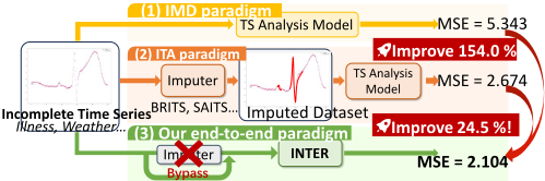
Existing Multivariate Time Series analysis methods are primarily designed for the full-knowledge scenario, which assumes access to completely observed datasets. For the IMTSA task, current solutions follow two flawed paradigms: (1) Ignoring missing data (IMD): Performing downstream analysis without addressing missing values, which leads to severely degraded performance. (2) Impute-then-analyze (ITSA): Imputing missing data before analysis, which suffers from redundant training and error accumulation, resulting in biased results and suboptimal performance.
Motivating Example. To better illustrate the challenges of incomplete multivariate time series analysis, we consider the widely used public medical dataset PhysioNet, which contains ICU patient records for tasks such as mortality prediction and clinical outcome analysis. Figure 1 compares the performance of existing paradigms for time series analysis on this dataset. The IMD paradigm that directly performs downstream analysis without handling missing values results in severely degraded performance. The ITSA paradigm first applies a standard imputation method (e.g., MICE [Buuren and Groothuis-Oudshoorn, 2010]) to fill in missing values, followed by a state-of-the-art model, such as a Transformerbased classifier [Lim and Zohren, 2021]. While this paradigm offers slight improvements, it suffers from error propagation introduced during the imputation phase, leading to biased analysis and suboptimal results.
To address the limitations of the above two paradigms, we propose a novel end-to-end framework, named INTER, which introduces a new paradigm for incomplete multivariate time series analysis by bypassing the imputation process. As shown in Figure 1(c), INTER directly analyzes incomplete time series data without requiring separate imputation. By eliminating error accumulation and effectively capturing missing patterns, INTER achieves significantly better accuracy and robustness results than existing paradigms.
However, implementing INTER faces two challenging problems. First, how can we effectively extract missing patterns and recover critical information from missing parts without performing explicit imputation? (CH1) The challenge lies in the fact that missing data patterns often exhibit complex temporal and spatial dependencies, making them difficult to model directly. Moreover, skipping the imputation step can render traditional feature extraction methods ineffective. Therefore, it is essential to design a mechanism capable of capturing both explicit and implicit missing patterns, which will enable accurate representation of incomplete time series. Second, how can we effectively adapt and transfer the knowledge derived from the missing data to diverse multivariate time series analysis tasks? (CH2) Incomplete time series occur across various downstream tasks, such as forecasting, anomaly detection, and imputation. When dealing with datasets with high missing rates, excessive noise in such datasets can prevent downstream time series analysis models from even bootstrapping effectively. Furthermore, different tasks require different utilizations of the missing information, and a lack of alignment mechanisms makes it difficult to adapt and fine-tune the missing information for each specific downstream task
To address these two challenges, INTER consists of two key modules: the missing-aware patch learning (MPL) module and the incomplete time series analysis (ITSA) module, each designed to tackle one of the challenges independently. In the MPL module, we devise a novel missing-rate-aware patch dropping (MPD) strategy and a missing-aware Transformer block, both of which we propose to enhance model generalization, robustness, and the ability to capture underlying patterns in the observed incomplete time series. In the ITSA module, we fine-tune a pre-trained language model (PLM) with a novel element-wise loss function. By leveraging the pre-trained knowledge from the PLM, ITSA captures the underlying structure of incomplete time series data and refines it using the element-wise loss function, which is designed to minimize the interference from noise in the missing data. This process enables INTER to effectively learn both the distributions of observed data and the missing state distributions from incomplete time series.
Our main contributions are as follows: (1) Paradigm: We propose INTER, an end-to-end, missing-aware framework for the IMTSA problem that bypasses imputation and achieves exceptional performance. To the best of our knowledge, this is the first attempt to develop an end-to-end framework for incomplete multivariate time series analysis. (2) Model: In INTER, we devise two novel modules, i.e., MPT based on missing-aware transformer and ITSA based on pretrain language model, to address the two challenges, respectively. (3) Theory: We propose a novel missing-state-aware patch-dropping (MPD) strategy and theoretically prove that MPD achieves lower sample variance for time series with the same dropout rate compared to other dropping strategies. (4) Experiment: We conduct extensive experiments on 11 realworld datasets, demonstrating that INTER outperforms stateof-the-art methods in terms of accuracy while maintaining comparable computational efficiency.
2 RelatedWork
Existing time series imputation models serve as the foundation for most multivariate time series analysis methods. They include statistical ones, attention-based ones, deep generative model based ones, and neural ordinary differential equation (NODE) based ones. In particular, the statistical time series imputation algorithms substitute missing values with the statistics, e.g., zero, mean, and last observed value or simple statistical models, including ARIMA [Bartholomew, 1971]. The attention mechanism based time series imputation methods contain TransI [Vaswani et al., 2017] and SAITS [Du et al., 2023]. The deep generative model based time series imputation methods use autoencoder and generative adversarial network to impute missing values, including BRITS [Cao et al., 2018] and CSDI [Tashiro et al., 2021]. The NODE-based methods model the dynamics over time by virtue of the continuous nature of NODE, such as SaShiMi [Goel et al., 2022] and LS4 [Zhou et al., 2023a].
Multivariate time series analysis methods have attracted extensive research focus from the AI community [Liang et al., 2024], and these approaches can be broadly categorized into three types. With the development of technologies such as Transformers, pretrained language models, and mixture of experts[Vaswani et al., 2017; Feng et al., 2024; Feng et al., 2025], Transformer-based models have become increasingly effective in time series analysis, including Informer [Zhou et al., 2021], PatchTST [Nie et al., 2022], OneFitsAll [Zhou et al., 2023b] and Timer[Liu et al., 2024]. The second category consists of non-Transformer-based models, such as CNN-based approaches like TimesNet [Wu et al., ] and TriD-MAE [Zhang et al., 2023], which capture spatial and temporal patterns using convolutions. With the development of GNN methods [Zhu et al., 2023; Liao et al., 2024], models like FourierGNN [Yi et al., 2023a] have started leveraging graph structures for multivariate time series forecasting. MLP-based models like FreTS [Yi et al., 2023b] and TSMixer [Ekambaram et al., 2023] focus on learning complex feature interactions in time series data. FilterNet [Yi et al., 2024] employs frequency filtering techniques to enhance forecasting performance. The third category involves diffusion-based models, such as D3VAE [Li et al., 2022] and DiffTime [Coletta et al., 2024], which model time series dynamics by progressively adding and removing noise, making them effective for handling missing or uncertain data.
3 ProblemDefinition
The input multivariate time series dataset contains a set of samples D = {X1, · · · ,XN} with d dimensions
MPL module
and L timestamps. Formally, X = (x1, · · · , xd)⊤ = (x:1, · · · , x:L) ∈ Rd×L with xi being (xi1, · · · , xiL). In particular, xij is the i-th feature value of X at the j-th timestamp, which is probably missing in the incomplete multivariate time series dataset.
Definition 1. Incomplete multivariate time series, IMTS. To encode the missing information of each sample X in D, a mask matrix M = (m1, · · · ,md)⊤ = (m:1, · · · ,m:L) ∈ {0, 1}d×L w.r.t. X is used to indicate whether the values in X exist or not. mi = (mi1, · · · ,miL), and mij being 0 or 1 means that, xij is missing or observed.
Definition 2. Incomplete multivariate time series representation learning, IMTSRL. Given an incomplete multivariate time series X with its mask matrix M, the goal of incomplete time series representation learning is to train a neural network model (i.e., encoder) f : Rd ↦→ Rdr , where dr is the dimensionality of the representation, such that the representation z = f(X) can be informative for downstream analysis tasks, e.g., multivariate time series classification.
Based on probability theory [Feng et al., 2023], we claim that, during model optimization, the analysis approach leveraging IMTSRL proves more effective than the imputationthen-analysis solution, as highlighted in Observation 1.
Framing the classification task as the foundation for IMTSRL, the objective is to train a classifier H that uses the IMTS data X ∈ D to predict the label y. For ease of representation, we restrict our domain to a three-class task in this part, i.e., y ∈ {0, 1, 2}. Inspired by [Feng et al., 2023], we evaluate the classifier's performance differences across various categories in the discrete attribute K in X that exhibits a complex missing mechanism, e.g., MAR and MNAR. Such a classifier is to solve a constrained optimization problem maxHE[I(H(X) = Y)] subject to Disc(H) ≤ ϵ, where ϵ ≥ 0 is a tolerance threshold. When the optimization is over binary mappings, the optimal solution of the constrained optimization problem only depends on the data distribution PK,X,Y and ϵ. We denote the optimal solution of this problem by Fϵ(PK,X,Y). Here, I is the indicator function, returning 1 if H correctly predicts H(X) = Y, and 0 otherwise. Disc(H) represents the model's disparity in performance across different categories in K, i.e., Disc(H) = maxy,ˆ y,k,k′ |Pr(H(X) = ˆ y | Y = y,K = k) - Pr(H(X) = ˆ y | Y = y,K = k′ )|. Moreover, we use mutual information [Kraskov et al., 2004] to quantify the dependence between the missing matrix M and the label Y, i.e., I(M;Y) ≜ ∑m∈M ∑y PM,Y(m, y) log PM,Y(m, y)/(PM(m)PY(y)). The detailed proof can be found in Appendix A.
Observation 1. Suppose that the incomplete IMTS dataset X with the mask matrix M and label set Y consists of a single discrete attribute K, which is subject to a complex missingness mechanism, such as MAR or MNAR. Let α represent the probability that the outcome of the three-class classification is not equal to 0 for a given sample. For any ϵ and α ∈ ( 12 , 1), there exists a data distribution PK,X,Y such that the optimal solution Fϵ(PK, ˆX,Y ) is less than or equal to the optimal solution Fϵ(PK,X,Y), i.e., supfimp Fϵ (PK, ˆX,Y ) ≤ Fϵ (PK,X,Y) - α, where fimp is the mapping function of the IMTS imputation model. The imputed data ˆX = fimp(X).
4 Methodology
4.1 Overall
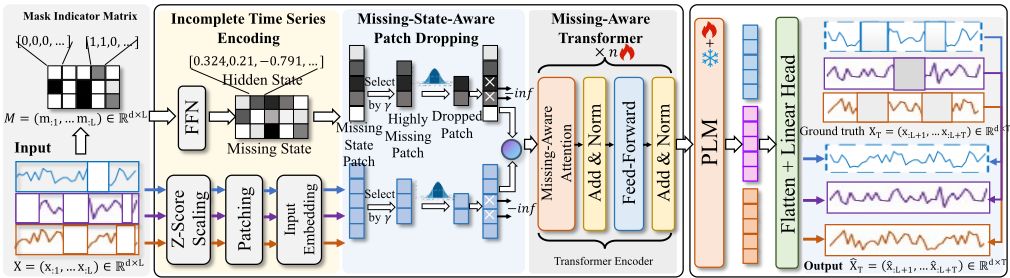
Our proposed INTER framework consists of two key modules: Missing-aware Patch Learning (MPL) and Incomplete Time Series Analysis (ITSA). The architecture of INTER is shown in Figure 2. Specifically, INTER takes an incomplete multivariate time series X = {x1, . . . , xL} ∈ Rd×L as input and processes it sequentially through the MPL and ITSA to generate outputs for downstream tasks. Figure 2 illustrates an example of the output for a time series forecasting task, ˆXT = {xL+1, . . . , xL+T}. First, the MPL module includes three components: incomplete time series encoding (TSE), missing-state-aware patch dropping (MPD), and missing-aware Transformer (MAT). TSE applies mainstream time series processing components for standard preprocessing and, moreover, learns the missing patterns in each incomplete multivariate time series. MPD adopts a novel patch-dropping strategy to reduce noise, enhancing model generalization and robustness. MAT learns the observed data distribution and the missing state distribution based on a
ITSA module
transformer-based encoder. Second, the ITSA module leverages pre-trained language models to provide prior knowledge for bootstrapping the learning of underlying observed time series patterns. It then uses a flattening layer and linear head to project the learned representations onto specific downstream tasks. Additionally, an element-wise loss function is introduced to mitigate the risk of learning incorrect information from missing values. The pseudo-code of INTER can be found in Appendix B.
4.2 MPL: Missing-aware Patch Learning
Traditional multivariate time series analysis models typically rely on imputation algorithms to handle missing data when performing IMTSA tasks. However, this paradigm introduces unnecessary training redundancy, error propagation, and ultimately leads to suboptimal performance. To address these issues, we propose the MPL module, which operates directly on incomplete multivariate time series, extracting patches containing missing values and observed time series data. This process enables the model to learn the underlying patterns of missing data and generate high-level hidden representations without imputation. Next, we elaborate on the three key components of the MPL module.
TSE: Incomplete Time Series Encoding. The TSE serves two primary purposes for processing incomplete time series data: (1) extracting missing state information and (2) generating embedded representations of the time series.
For the first purpose, TSE employs a feedforward neural network (FFN) to extract the missing-state matrix Ms ∈ Rd×L from the mask indicator matrix M ∈ {0, 1}d×L. To achieve this, the mask indicator matrix is divided into patches P , which are then passed through the FFN to learn the missing state matrix, where for the i-th patch, the missing state ms,p i = fFFN(mpi ). This learned missing state is then used in the MPD module to provide a missing pattern of each patch for further refinement.
For the second purpose, TSE first normalizes the incomplete time series using Z-score scaling. Specifically, for each time series xi ∈ X with its corresponding mask vector mi ∈ M, we calculate the mean µi and standard deviation σi across the observed elements, i.e.,
Then, for each observed value in xi, we subtract µi and divide by σi. This normalization reduces variability, promoting stable learning across the data. Note that a de-normalization procedure is applied to the forecasted data to ensure that the predicted time series are interpretable in relation to the historical data. After normalization, we divide the time series into non-overlapping patches ¨xpi ∈ RP×N , where each patch corresponds to a subseries-level segment of the time series [Nie et al., 2022]. Finally, we apply an Input Embedding layer to project the time series embedding ¨xpi to xpi , where xpi is mapped to the required dimensions for the subsequent pre-trained model [Zhou et al., 2023b]. This embedding captures complex dependencies across time steps and is crucial for facilitating the learning process in later modules.
MPD: Missing-state-aware patch dropping. The core idea of the MPD is to perform dropping based on the missing states of the time series data. Unlike traditional dropout methods, which apply a uniform dropping probability across all data points, MPD introduces a random incomplete patch dropping strategy. This strategy directly applies dropping to incomplete time series patches, rather than individual time series values. Specifically, MPD drops incomplete time series patches at a rate of δ, such that, on average, δ · P patches are masked in each time series. Moreover, the dropping probability δp i for each patch is dynamically determined based on its missing rate γ p i , with patches that have a higher proportion of missing data being more likely to be dropped due to the significant noise they carry.
The dropping operation in MPD can be viewed as a patchsampling process. For each patch xpi in the time series, an independent mask αi is generated to determine whether the patch will be preserved, following a Bernoulli distribution:
where δp is the dropping probability dynamically assigned to each patch xpi , based on its missing rate γ p . Specifically, the dropping probability δp for each patch is designed to be positively correlated with its missing rate γ p , such that:
where f (γ p ) is a function that increases with the patch's missing rate, enabling an adaptive dropping strategy that effectively addresses the challenges posed by patches containing a high proportion of missing values. Subsequently, for each patch xpi and its corresponding missing state ms,p i , the mask αi is generated based on the Bernoulli distribution with the dropping probability δp . Finally, the perturbed time series matrix is obtained by performing element-wise multiplication of each patch with its corresponding mask αi.
The effectiveness and theoretical advantages of the MPD strategy are demonstrated through rigorous analysis. Specifically, Theorem 1 shows that the MPD strategy based on missing rates results in lower sample variance at the same dropout rate, contributing to a more stable training process. Therefore, the MPD strategy can serve as an additional regularization term of INTER, thereby improving the model's robustness. The detailed proof can be found in Appendix C.
Theorem 1. Compared to two existing dropping strategies, i,e, (i) a value-based dropping strategy, and (ii) a random patch-dropping strategy based on uniform distribution, the MPD strategy achieves a smaller sample variance on time series with the same dropout rate.
MAT: Missing-aware Transformer. The MAT module leverages an n-layer Transformer to process missing stateaware patches and time series patches, capturing hidden temporal patterns and producing a sequence of hidden representations {zi}Ni=1 that integrate both observed data and missing state information.
First, the time series vector xpi and the corresponding missing state ms,p i are concatenated to form a combined representation for each patch, i.e., zpi = concat(xpi ,ms,p i ). This embeds the missing state distribution into the time series patches, enriching the input representation with information about both observed data and missing patterns.
Next, during the self-attention computation, patches marked as dropped need to be excluded by masking their attention scores. Therefore, we devise a missing-aware attention with a new score-updating mechanism. Specifically, given the attention score matrix A ∈ RN×N , the scores are updated as follows:
where D is the dropped data. This ensures that dropped patches do not influence the attention mechanism, focusing the model only on valid patches.
Finally, the remaining patches are passed through the Transformer, which performs missing-aware self-attention and feedforward operations to generate the hidden representation for each patch, i.e., ˜zpi = Transformer({zpj | j /∈ D}). This enables the Transformer to aggregate temporal dependencies across patches while incorporating missing state information into the learned representations. The MAT module outputs the sequence of hidden representations ˜Zp = {˜zpi }P-|D| i=1 , where each vector effectively encodes both observed time series data and missing state information, providing a robust foundation for downstream tasks.
4.3 ITSA: Incomplete Time Series Analysis
After the MPL module, INTER employs the incomplete time series analysis (ITSA) module, which processes each patch independently in a sequence-to-sequence framework. ITSA leverages pre-trained parameters from NLP models, specifically GPT-2 [Radford et al., 2019], to enhance the representation of incomplete time series data.
Architecture. In ITSA, time series patches ˜Zp fromMPL are treated as sequence tokens and passed through the pretrained language model (PLM). ITSA retains the PLM's positional embeddings and self-attention blocks. As most knowledge resides in the self-attention and FFN layers, these are frozen during fine-tuning, allowing only final layers to adapt and better capture temporal dependencies in time series data.
Specifically, the input to ITSA is a sequence of patches ˜Zp . The PLM processes this as: H = PLM(˜Zp ), where H ∈ RN×D is the output hidden representation and D is the PLM hidden size. GPT-2 is used as the PLM in our experiments. During fine-tuning, only the output layers are updated, while self-attention and FFN remain frozen. The output H captures complex temporal patterns from incomplete multivariate time series. ITSA is designed to leverage PLM knowledge to model incomplete structures. Fine-tuning on incomplete patches improves the model's ability to learn latent temporal dependencies, helping INTER better handle missing values and uncover hidden patterns for downstream tasks.
Objective. On top of PLM, ITSA applies a flatten layer (FL) and a linear head (LH) to infer future time series: ˆxTi = (ˆx1i , · · · , ˆxdi ) = FL(LH(H)). where H is the ITSA output. Moreover, the ITSA module incorporates distinct objective functions specifically designed for various tasks, including forecasting (both long-term and short-term), anomaly detection, and imputation on incomplete time series data. Taking the incomplete time series forecasting task as an example, the ITSA module is designed to effectively learn the mapping between incomplete historical time series and future observations. To achieve this, we propose an incomplete time series Mean Squared Error (MSE) loss function, defined as:
where ⊙ is the element-wise multiplication. || · ||22 represents the squared Euclidean norm, which is the sum of the squares of the elements of a vector. xTi is the ground-truth future data of the time series xi ∈ X. mTi in MT is the mask vector w.r.t. xTi . The incomplete time series forecasting loss function LMSE is designed to enforce the consistency between the true underlying data distribution in incomplete future time series and output data distribution. It can be easily generalized to other time series analysis tasks, e.g., the incomplete time series classification, as described in Appendix D.
5 Experiment
In this section, we evaluate the performance of our proposed model INTER on five tasks-long-term forecasting, shortterm forecasting, imputation, classification, and anomaly detection-using 11 (in)complete multivariate time series datasets. The performance is compared with a total of 8 stateof-the-art time series analysis methods. All approaches were implemented in Python. The experiments were conducted on a server with an Intel Core 2.80GHz processor, 3 NVIDIA A40 GPUs, and 192GB RAM, running Ubuntu 18.04.
5.1 Experiment Settings
Metrics. We evaluate the effectiveness of models in time series forecasting tasks using the mean square error (MSE) and mean absolute error (MAE), where smaller metric values indicate better prediction performance. For time series classification tasks, we use Accuracy as the evaluation metric to measure model effectiveness. To evaluate the effectiveness of forecasting models on incomplete multivariate time series datasets, we randomly remove 50% of the observed values prior to model training. Each metric value is obtained by averaging the results of five experimental runs on each dataset.
Baselines. In the experiments, the baselines include six state-of-the-art time series forecasting methods, including: Informer [Zhou et al., 2021], PatchTST [Nie et al., 2022], TimesNet [Wu et al., ], OneFitsAll [Zhou et al., 2023b], Timer [Liu et al., 2024], and TriD-MAE [Zhang et al., 2023]. Since almost all the above baselines cannot be trained with incomplete time series data, we employ five state-of-the-art multivariate time series imputation methods, i.e., Zero [Che et al., 2018], BRITS [Cao et al., 2018], TransI [Vaswani et al., 2017], SAITS [Du et al., 2023], and CSDI [Tashiro et al., 2021] to impute missing values.
5.2 Comparison Study
Overall, the proposed method, INTER, outperforms other models across various tasks, including incomplete time series long-term and short-term forecasting, classification, anomaly detection, and imputation. Due to space limitations, the experimental results for anomaly detection and imputation tasks are presented in Appendix E.1. These results highlight the effectiveness and robustness of the proposed INTER framework in handling incomplete time series data.
| Models | Electricity | Weather | Exchange | Illness | ||||
|---|---|---|---|---|---|---|---|---|
| MSE | MAE | MSE | MAE | MSE | MAE | MSE | MAE | |
| Informer Zero BRITS TransI SAITS CSDI | 0.352 ± 0.012 0.358 ± 0.006 0.356 ± 0.015 0.352 ± 0.01 \ | 0.428 ± 0.009 0.434 ± 0.004 0.432 ± 0.015 0.430 ± 0.007 \ | 0.463 ± 0.001 0.514 ± 0.007 0.462 ± 0.014 0.510 ± 0.019 \ | 0.458 ± 0.012 0.480 ± 0.005 0.444 ± 0.009 0.475 ± 0.016 \ | 0.524 ± 0.007 0.522 ± 0.005 0.504 ± 0.009 0.549 ± 0.001 0.508 ± 0.006 | 0.564 ± 0.003 0.576 ± 0.007 0.570 ± 0.005 0.588 ± 0.009 0.570 ± 0.001 | 5.706 ± 0.123 5.552 ± 0.456 5.168 ± 0.789 5.706 ± 0.012 5.278 ± 0.345 | 1.480 ± 0.051 1.591 ± 0.032 1.510 ± 0.076 1.616 ± 0.091 1.532 ± 0.043 |
| PatchTST | Zero 0.222 ± BRITS 0.201 ± TransI 0.207 ± SAITS 0.198 ± CSDI | 0.018 0.320 ± 0.018 0.02 0.299 ± 0.012 0.01 0.303 ± 0.016 0.018 0.296 ± 0.008 \ | 0.201 ± 0.015 0.146 ± 0.01 0.163 ± 0.003 0.143 ± 0.012 \ | 0.279 ± 0.007 0.190 ± 0.014 0.204 ± 0.018 0.181 ± 0.01 \ | 0.582 ± 0.008 0.143 ± 0.003 0.362 ± 0.012 0.266 ± 0.004 0.05 ± 0.007 | 0.580 ± 0.004 0.288 ± 0.008 0.471 ± 0.006 0.367 ± 0.003 0.156 ± 0.002 | 3.943 ± 0.678 2.729 ± 0.901 3.024 ± 0.234 2.520 ± 0.567 8.191 ± 3.191 | 1.402 ± 0.025 1.104 ± 0.087 1.216 ± 0.036 1.052 ± 0.019 1.640 ± 0.057 |
| TimesNet Zero BRITS TransI SAITS CSDI | \ 0.202 ± 0.014 0.175 ± 0.019 0.183 ± 0.02 0.172 ± 0.012 \ | 0.311 ± 0.014 0.284 ± 0.019 0.289 ± 0.002 0.282 ± 0.006 \ | 0.473 ± 0.004 0.144 ± 0.017 0.159 ± 0.002 0.144 ± 0.009 \ | 0.480 ± 0.015 0.198 ± 0.017 0.213 ± 0.004 0.196 ± 0.009 \ | 0.978 ± 0.004 0.194 ± 0.009 0.408 ± 0.011 0.114 ± 0.005 0.061 ± 0.008 | 0.753 ± 0.01 0.352 ± 0.007 0.508 ± 0.004 0.263 ± 0.005 0.180 ± 0.001 | 5.253 ± 0.135 3.949 ± 0.246 4.436 ± 0.369 3.926 ± 0.789 7.140 ± 0.012 | 1.620 ± 0.049 1.366 ± 0.067 1.499 ± 0.008 1.354 ± 0.099 1.805 ± 0.027 |
| OneFisAll Zero BRITS TransI SAITS CSDI | 0.267 ± 0.01 0.213 ± 0.017 0.219 ± 0.012 0.21 ± 0.02 \ | 0.359 ± 0.011 0.301 ± 0.014 0.305 ± 0.005 0.296 ± 0.019 \ | 0.277 ± 0.005 0.159 ± 0.016 0.175 ± 0.007 0.159 ± 0.011 \ | 0.361 ± 0.001 0.206 ± 0.008 0.217 ± 0.019 0.198 ± 0.006 \ | 0.720 ± 0.006 0.133 ± 0.003 0.366 ± 0.007 0.083 ± 0.01 0.052 ± 0.001 | 0.677 ± 0.009 0.291 ± 0.008 0.487 ± 0.006 0.216 ± 0.003 0.161 ± 0.002 | 5.009 ± 0.395 3.579 ± 0.678 3.287 ± 0.901 4.328 ± 0.234 6.455 ± 0.567 | 1.571 ± 0.041 1.421 ± 0.056 1.308 ± 0.013 1.531 ± 0.078 1.638 ± 0.009 |
| Timer Zero BRITS TransI SAITS CSDI | 0.272 ± 0.016 0.186 ± 0.013 0.193 ± 0.002 0.167 ± 0.016 \ | 0.378 ± 0.016 0.281 ± 0.007 0.285 ± 0.003 0.267 ± 0.015 \ | 0.290 ± 0.019 0.179 ± 0.003 0.215 ± 0.008 0.184 ± 0.015 \ | 0.411 ± 0.007 0.236 ± 0.014 0.260 ± 0.018 0.212 ± 0.005 \ | 0.800 ± 0.004 0.173 ± 0.008 0.386 ± 0.002 0.059 ± 0.006 0.053 ± 0.007 | 0.737 ± 0.007 0.311 ± 0.001 0.457 ± 0.005 0.188 ± 0.01 0.196 ± 0.012 | 5.343 ± 0.89 3.549 ± 0.135 3.337 ± 0.246 2.674 ± 0.369 4.288 ± 0.789 | 1.720 ± 0.083 1.461 ± 0.045 1.318 ± 0.015 1.091 ± 0.06 1.501 ± 0.031 |
| TriD-MAE | 0.311 ± 0.018 | 0.391 ± 0.004 | 0.233 ± 0.027 0.322 ± 0.091 | 1.388 ± 0.200 | 0.940 ± 0.009 | 8.290 ± 0.012 | 2.170 ± 0.092 | |
| INTER (Ours) | 0.147 ± 0.01 | 0.250 ± 0.018 | 0.139 ± 0.017 0.192 ± 0.020 | 0.049 ± 0.003 | 0.158 ± 0.013 | 2.104 ± 0.345 | 0.984 ± 0.007 | |
In addition, we investigate the influence of different elements of INTER on the prediction performance over the incomplete multivariate time series data, i.e., Ablation Study. The detailed experimental results are described in Appendix E.2. We can observe that, each component of INTER positively affects performance. Then, we study the Effect of Missing Rate (i.e., how many features/values in multivariate time series data are dropped) on the time series analysis performance. The detailed experimental results are described in Appendix E.3. One can observe that, INTER basically achieves the best forecasting performance in each case.
Incomplete Long-term Time Series Forecasting
Setups. To fully evaluate model performance in forecasting, we adopt two benchmark types: long-term and short-term. For the long-term setting, we use four widely-used public multivariate time series datasets: Electricity [Gasparin et al., 2022], Weather [Zhou et al., 2021], Exchange [Zhang and Berardi, 2001], and Illness [Zhou et al., 2021], covering four real-world scenarios.
Results. Table 1 presents the experimental results of incomplete time series forecasting methods. For Electricity and Weather, results of CSDI-based baselines are unavailable (denoted as "\") due to exceeding the 105 -second time limit.
| Models | M4-Yearly | M4-Monthly | |||
|---|---|---|---|---|---|
| SMAPE | MASE | SMAPE | MASE | ||
| TimesNet | Zero SAITS | 18.523 15.460 | 7.512 5.079 | 17.421 14.371 | 2.980 1.922 |
| OneFitsAll | Zero SAITS | 17.531 15.419 | 7.015 5.033 | 17.283 14.320 | 4.965 1.870 |
| Timer | Zero SAITS | 18.586 15.510 | 7.180 5.124 | 17.491 14.478 | 5.046 1.982 |
| INTER (Ours) | \ | 15.322 | 4.913 | 14.106 | 1.790 |
This is caused by the much higher complexity of CSDI's score-based diffusion model compared to other imputation methods.
It can be observed that INTER substantially outperforms all baselines. In forecasting accuracy (MSE and MAE), INTER surpasses the best imputation-based method (Timer with SAITS) by 20.91% on average, reaching 24.46% on Illness in terms of MSE. Compared to TriD-MAE, which integrates built-in imputation, INTER achieves an average improvement of 76.20% in MSE, demonstrating a significant accuracy gain. This is attributed to INTER's use of an effective analysis model that combines a missing-state-aware dropping strategy with an incomplete forecasting loss, thus boosting accuracy.
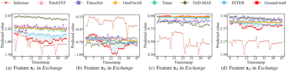
Visualization. Figure 3 visualizes forecasting results for the top 4 features of a randomly selected sample from Exchange. It clearly shows that INTER yields much better accuracy than baselines, consistently being closest to the ground truth, further confirming its strong forecasting ability on incomplete multivariate time series.
| Models | Impu. | Physionet | Heartbeat | JapaneseVowels |
|---|---|---|---|---|
| Informer 2021 | Zero BRITS SAITS | 0.774 0.786 0.803 | 0.724 0.730 0.735 | 0.904 0.962 0.962 |
| PatchTST 2022 | Zero BRITS SAITS | 0.867 0.877 0.875 | 0.780 0.737 0.780 | 0.910 0.965 0.964 |
| Dlinear 2023 | Zero BRITS SAITS | 0.769 0.782 0.797 | 0.717 0.722 0.727 | 0.874 0.912 0.929 |
| TimesNet 2023 | Zero BRITS SAITS | 0.865 0.878 | 0.722 0.751 0.756 | 0.906 0.964 0.963 |
| OneFitsAll 2023 | Zero BRITS SAITS | 0.874 | 0.728 0.761 0.757 | 0.912 0.966 |
| Timer 2024 | Zero BRITS SAITS | 0.873 0.886 0.882 0.872 0.885 0.881 | 0.734 0.767 0.763 | 0.965 0.876 0.914 0.931 |
| TriD-MAE | \ | 0.776 | 0.723 | 0.856 |
| \ | 0.897 | 0.820 | 0.989 | |
| INTER (Ours) |
Incomplete Short-term Time Series Forecasting
Setups. For the short-term setting, we adopt the M4 [Makridakis, 2018] dataset and its representative subsets, including yearly and monthly collected univariate marketing data. The M4 dataset contains 100,000 time series at varying frequencies. We adopt three baselines with strong performance on this task: TimesNet, OneFitsAll, and Timer. For each imputethen-analysis method, we use two representative imputation algorithms, Zero and SAITS, to fill in the missing data.
Results. Table 2 presents the experimental results of multivariate time series analysis methods for the short-term forecasting task. It can be observed that INTER clearly outperforms all baselines, exceeding the best-performing method (i.e., OneFitsAll with SAITS) by an average of 2.90%, demonstrating its strong capability in short-term forecasting tasks.
Incomplete Time Series Classification
Setups. We adopt sequence-level classification to verify the model's capacity for high-level representation learning. We use three public real-world time series datasets: two representative multivariate datasets from the UEA Time Series Classification Archive [Bagnall et al., 2018] (i.e., Heartbeat and JapaneseVowels), and one public medical dataset (i.e., Physionet) [Goldberger et al., 2000]. We pre-process the datasets following the descriptions in [Zerveas et al., 2021], where subsets vary in sequence length.
Results. Table 3 presents a comparative analysis of classification performance across the three datasets. INTER achieves the best performance in all cases, surpassing the best baseline, OneFitsAll with BRITS, by an average of 3.56% in accuracy. Compared with the analysis method incorporating built-in imputation, TriD-MAE, INTER achieves an average improvement of 14.91% in accuracy. Moreover, INTER demonstrates the most stable classification accuracy, further validating its effectiveness.
6 Conclusion
In this paper, we propose INTER, a novel end-to-end framework for incomplete multivariate time series analysis that bypasses traditional imputation methods by leveraging PLM to directly learn the distribution of incomplete time series data. We further provide a theoretical analysis showing that the MPD strategy in INTER achieves lower sample variance for time series with the same dropout rate compared to alternative dropping strategies, demonstrating its statistical advantage. Extensive experiments conducted on 11 publicly available real-world time series datasets show that INTER greatly beats the state-of-the-art methods in effectiveness.
Acknowledgments
This work was supported in part by the "Pioneer" and "Leading Goose" R&D Program of Zhejiang (No. 2024C01212), and the Ningbo Yongjiang Talent Programme Grant 2024A158-G. Mengyin Zhu is the corresponding author of the work.
@inproceedings{ijcai2025p734,
  title     = {General Incomplete Time Series Analysis via Patch Dropping Without Imputation},
  author    = {Wu, Yangyang and Yuan, Yi and Zhu, Mengying and Miao, Xiaoye and Xi, Meng},
  booktitle = {Proceedings of the Thirty-Fourth International Joint Conference on
               Artificial Intelligence, {IJCAI-25}},
  publisher = {International Joint Conferences on Artificial Intelligence Organization},
  editor    = {James Kwok},
  pages     = {6597--6605},
  year      = {2025},
  month     = {8},
  note      = {Main Track},
  doi       = {10.24963/ijcai.2025/734},
  url       = {https://doi.org/10.24963/ijcai.2025/734},
}
TY - CPAPER TI - General Incomplete Time Series Analysis via Patch Dropping Without Imputation AU - Wu, Yangyang AU - Yuan, Yi AU - Zhu, Mengying AU - Miao, Xiaoye AU - Xi, Meng T2 - Proceedings of the Thirty-Fourth International Joint Conference on Artificial Intelligence, IJCAI-25 PB - International Joint Conferences on Artificial Intelligence Organization PY - 2025 SP - 6597 EP - 6605 DO - 10.24963/ijcai.2025/734 UR - https://doi.org/10.24963/ijcai.2025/734 ER -Copied
Machine-readable versions of this paper, for tools and AI agents:





