
Continuous Diffusive Prediction Network for Multi-Station Weather Prediction
Proceedings of the Thirty-Fourth International Joint Conference on Artificial Intelligence. Main Track. Pages 6714-6722.
https://doi.org/10.24963/ijcai.2025/747
Keywords
- Machine Learning: ML: Time series and data streams
- Multidisciplinary Topics and Applications: MTA: Other
- Machine Learning: ML: Applications
Abstract
Multi-station weather prediction provides weather forecasts for specific geographical locations, playing an important role in various aspects of daily life. Existing methods consider the relationships between individual stations discretely, making it difficult to model the continuous spatiotemporal processes of atmospheric motion, which results in suboptimal prediction outcomes. This paper proposes the Continuous Diffusive Prediction Network (CDPNet) to model the real-world continuous weather change process from discrete station observation data. CDPNet consists of two core modules: the Continuous Calibrated Initialization (CCI) and the Diffusive Difference Estimation (DDE). The CCI module interpolates data between observation stations to construct a spatially continuous physical field and ensures temporal continuity by integrating directional information from a global perspective. It accurately represents the current physical state and provides a foundation for future weather prediction. Moreover, the DDE module explicitly captures the spatial diffusion process and estimates the diffusive differences between consecutive time steps, effectively modeling spatio-temporally continuous atmospheric motion. Likewise, directional information on weather changes is introduced from the entire historical series to mitigate estimation uncertainty and improve the performance of weather prediction. Extensive experiments on the Weather2K and Global Wind/Temp datasets demonstrate that CDPNet outperforms state-of-the-art models.
- [Bauer et al., 2015] Peter Bauer, Alan Thorpe, and Gilbert Brunet. The quiet revolution of numerical weather pre- diction. Nature, 525(7567):47-55, 2015.
- [Bhattacharyya et al., 2022] M Bhattacharyya, S Nag, and U Ghosh. Deciphering environmental air pollution with large scale city data. In Proceedings of the Thirty-First International Joint Conference on Artificial Intelligence, 2022. IJCAI
- [Bi et al., 2023] Kaifeng Bi, Lingxi Xie, Hengheng Zhang, Xin Chen, Xiaotao Gu, and Qi Tian. Accurate medium- range global weather forecasting with 3d neural networks. Nature, 619(7970):533-538, 2023.
- [Chen et al., 2018] Ricky TQ Chen, Yulia Rubanova, Jesse Bettencourt, and David K Duvenaud. Neural ordinary dif- ferential equations. Advances in neural information pro- cessing systems, 31, 2018.
- [Chen et al., 2024] Shengchao Chen, Guodong Long, Tao Shen, Jing Jiang, and Chengqi Zhang. Federated prompt learning for weather foundation models on devices. In Proceedings of the Thirty-Third International Joint Con- ference on Artificial Intelligence, IJCAI 2024, Jeju, South Korea, August 3-9, 2024, pages 5772-5780. ijcai.org, 2024. IJCAI
- [Feng et al., 2024] Yutong Feng, Qiongyan Wang, Yutong Xia, Junlin Huang, Siru Zhong, and Yuxuan Liang. Spatio- temporal field neural networks for air quality inference. In Proceedings of the Thirty-Third International Joint Con- ference on Artificial Intelligence, IJCAI 2024, Jeju, South Korea, August 3-9, 2024, pages 7260-7268. ijcai.org, 2024.
- [Gravina et al., 2024] Alessio Gravina, Daniele Zambon, Davide Bacciu, and Cesare Alippi. Temporal graph odes for irregularly-sampled time series. In Proceedings of the Thirty-Third International Joint Conference on Artificial Intelligence, IJCAI 2024, Jeju, South Korea, August 3-9, 2024, pages 4025-4034. ijcai.org, 2024. IJCAI
- [Guen and Thome, 2020] Vincent Le Guen and Nicolas Thome. Disentangling physical dynamics from unknown factors for unsupervised video prediction. In Proceedings of the IEEE/CVF conference on computer vision and pat- tern recognition, pages 11474-11484, 2020.
- [Guo et al., 2019] Shengnan Guo, Youfang Lin, Ning Feng, Chao Song, and Huaiyu Wan. Attention based spatial- temporal graph convolutional networks for traffic flow forecasting. In Proceedings of the AAAI conference on artificial intelligence, volume 33, pages 922-929, 2019.
- [Han et al., 2023] Jindong Han, Hao Liu, Hengshu Zhu, and Hui Xiong. Kill two birds with one stone: A multi-view multi-adversarial learning approach for joint air quality and weather prediction. IEEE Transactions on Knowledge and Data Engineering, 35(11):11515-11528, 2023.
- [He et al., 2020] Zhanjun He, Min Deng, Jiannan Cai, Zhong Xie, Qingfeng Guan, and Chao Yang. Mining spa- tiotemporal association patterns from complex geographic phenomena. International Journal of Geographical Infor- mation Science, 34(6):1162-1187, 2020.
- [Kochkov et al., 2024] Dmitrii Kochkov, Janni Yuval, Ian Langmore, Peter Norgaard, Jamie Smith, Griffin Mooers, Milan Klöwer, James Lottes, Stephan Rasp, Peter Düben, et al. Neural general circulation models for weather and climate. Nature, pages 1-7, 2024.
- [Li et al., 2018] Yaguang Li, Rose Yu, Cyrus Shahabi, and Yan Liu. Diffusion convolutional recurrent neural net- work: Data-driven traffic forecasting. In International Conference on Learning Representations, 2018.
- [Lin et al., 2022] Haitao Lin, Zhangyang Gao, Yongjie Xu, Lirong Wu, Ling Li, and Stan Z Li. Conditional local convolution for spatio-temporal meteorological forecast- ing. In Proceedings of the AAAI conference on artificial intelligence, volume 36, pages 7470-7478, 2022.
- [Liu et al., 2024] Yong Liu, Chenyu Li, Jianmin Wang, and Mingsheng Long. Koopa: Learning non-stationary time series dynamics with koopman predictors. Advances in Neural Information Processing Systems, 36, 2024.
- [Ma et al., 2023] Minbo Ma, Peng Xie, Fei Teng, Bin Wang, Shenggong Ji, Junbo Zhang, and Tianrui Li. Histgnn: Hierarchical spatio-temporal graph neural network for weather forecasting. Information Sciences, 648:119580, 2023.
- [Mao et al., 2024] Rui Mao, Qika Lin, Qiawen Liu, Gian- marco Mengaldo, and Erik Cambria. Understanding pub- lic perception towards weather disasters through the lens of metaphor. In Proceedings of the thirty-third interna- tional joint conference on artificial intelligence, 2024. IJCAI
- [Salehizadeh et al., 2024] Mohammad Reza Sale- hizadeh, Ays ¸e Kübra Erenoglu, İbrahim S ¸engör, Akın Tas ¸cıkaraoglu, Ozan Erdinc ¸, Jay Liu, and João PS Catalão. Preventive energy management strategy before extreme weather events by modeling evs' opt-in preferences. IEEE Transactions on Intelligent Transportation Systems, 2024.
- [Schirmer et al., 2022] Mona Schirmer, Mazin Eltayeb, Ste- fan Lessmann, and Maja Rudolph. Modeling irregular time series with continuous recurrent units. In Inter- national conference on machine learning, pages 19388- 19405. PMLR, 2022.
- [Seo et al., 2018] Youngjoo Seo, Michaël Defferrard, Pierre Vandergheynst, and Xavier Bresson. Structured sequence modeling with graph convolutional recurrent networks. In Neural Information Processing: 25th International Con- ference, ICONIP 2018, Siem Reap, Cambodia, Decem- ber 13-16, 2018, Proceedings, Part I 25, pages 362-373. Springer, 2018.
- [Shepard, 1968] Donald Shepard. A two-dimensional inter- polation function for irregularly-spaced data. In Proceed- ings of the 1968 23rd ACM national conference, pages 517-524, 1968.
- [Tabar et al., 2022] Maryam Tabar, Dongwon Lee, David P Hughes, and Amulya Yadav. Mitigating low agricultural productivity of smallholder farms in africa: Time-series forecasting for environmental stressors. In Proceedings of the AAAI Conference on Artificial Intelligence, volume 36, pages 12608-12614, 2022.
- [Tang et al., 2024] Jiabin Tang, Wei Wei, Lianghao Xia, and Chao Huang. Easyst: A simple framework for spatio- temporal prediction. In Proceedings of the 33rd ACM International Conference on Information and Knowledge Management, pages 2220-2229, 2024.
- [Wang et al., 2024a] Peixiao Wang, Tong Zhang, Hengcai Zhang, Shifen Cheng, and Wangshu Wang. Adding atten- tion to the neural ordinary differential equation for spatio- temporal prediction. International Journal of Geographi- cal Information Science, 38(1):156-181, 2024.
- [Wang et al., 2024b] Yiyang Wang, Yuchen Han, and Yuhan Guo. Self-adaptive extreme penalized loss for imbalanced time series prediction. In Proceedings of the Thirty-Third International Joint Conference on Artificial Intelligence, IJCAI 2024, Jeju, South Korea, August 3-9, 2024, pages 5135-5143. ijcai.org, 2024. IJCAI
- [Wu et al., 2021] Haixu Wu, Jiehui Xu, Jianmin Wang, and Mingsheng Long. Autoformer: Decomposition transform- ers with auto-correlation for long-term series forecast- ing. Advances in neural information processing systems, 34:22419-22430, 2021.
- [Wu et al., 2023] Haixu Wu, Hang Zhou, Mingsheng Long, and Jianmin Wang. Interpretable weather forecasting for worldwide stations with a unified deep model. Nature Ma- chine Intelligence, 5(6):602-611, 2023.
- [Wu et al., 2024] Binqing Wu, Weiqi Chen, Wengwei Wang, Bingqing Peng, Liang Sun, and Ling Chen. Weathergnn: Exploiting meteo-and spatial-dependencies for local nu- merical weather prediction bias-correction. In Proceed- ings of the International Joint Conference on Artificial In- telligence, pages 2433-2441, 2024. IJCAI
- [Xu et al., 2024] Zhewen Xu, Xiaohui Wei, Jieyun Hao, Junze Han, Hongliang Li, Changzheng Liu, Zijian Li, Dongyuan Tian, and Nong Zhang. Dgformer: a physics- guided station level weather forecasting model with dy- namic spatial-temporal graph neural network. GeoInfor- matica, pages 1-35, 2024.
- [Yan et al., 2023] Xusheng Yan, Yaodeng Chen, Gang Ma, Luyao Qin, Peng Zhang, and Xinya Gong. A 3d cloud de- tection method for fy-4a giirs and its application in opera- tional numerical weather prediction system. IEEE Trans- actions on Geoscience and Remote Sensing, 2023.
- [Zhang et al., 2023] Yuchen Zhang, Mingsheng Long, Kaiyuan Chen, Lanxiang Xing, Ronghua Jin, Michael I Jordan, and Jianmin Wang. Skilful nowcasting of extreme precipitation with nowcastnet. Nature, 619(7970):526- 532, 2023.
- [Zheng et al., 2023] Xiangtao Zheng, Haowen Cui, Chujie Xu, and Xiaoqiang Lu. Dual teacher: A semisuper- vised cotraining framework for cross-domain ship detec- tion. IEEE Transactions on Geoscience and Remote Sens- ing, 61:1-12, 2023.
- [Zhou et al., 2021] Haoyi Zhou, Shanghang Zhang, Jieqi Peng, Shuai Zhang, Jianxin Li, Hui Xiong, and Wan- cai Zhang. Informer: Beyond efficient transformer for long sequence time-series forecasting. In Proceedings of the AAAI conference on artificial intelligence, volume 35, pages 11106-11115, 2021.
- [Zhou et al., 2022] Tian Zhou, Ziqing Ma, Qingsong Wen, Xue Wang, Liang Sun, and Rong Jin. Fedformer: Fre- quency enhanced decomposed transformer for long-term series forecasting. In International conference on machine learning, pages 27268-27286. PMLR, 2022.
- [Zhou et al., 2024] Ziyu Zhou, Gengyu Lyu, Yiming Huang, Zihao Wang, Ziyu Jia, and Zhen Yang. Sdformer: Trans- former with spectral filter and dynamic attention for mul- tivariate time series long-term forecasting. In Proceedings of the Thirty-Third International Joint Conference on Ar- tificial Intelligence, pages 3-9, 2024. IJCAI
- [Zhu et al., 2023] Xun Zhu, Yutong Xiong, Ming Wu, Gaozhen Nie, Bin Zhang, and Ziheng Yang. Weather2k: A multivariate spatio-temporal benchmark dataset for mete- orological forecasting based on real-time observation data from ground weather stations. In International Conference on Artificial Intelligence and Statistics, pages 2704-2722.
- PMLR, 2023.
References were extracted automatically from the PDF and may contain errors.
Full text extracted automatically from the PDF; figures, tables and equations may differ. The PDF is the version of record.
1 Introduction
Weather prediction plays a vital role in our life by providing crucial information for disaster preparedness [Mao et al., 2024], agricultural planning [Tabar et al., 2022], transportation safety [Zheng et al., 2023], energy management [Salehizadeh et al., 2024], and environmental protection [Bhattacharyya et al., 2022], etc. Multi-station weather prediction incorporates spatial correlations across regional stations, providing enhanced forecasting accuracy and regional flexibility, making it an important focus in modern meteorological research [Wu et al., 2023]. Traditional multi-station weather prediction typically relies on Numerical Weather Prediction (NWP) methods [Bauer et al., 2015; Yan et al., 2023; Wu et al., 2024], which use mathematical models to simulate atmospheric processes based on fundamental principles of physics and fluid dynamics. While NWP methods can produce regularly updated forecasts by solving complex equations, they require substantial computational resources and are constrained by the quality and coverage of observational data. In recent years, deep learning based weather prediction methods [Lin et al., 2022; Ma et al., 2023; Han et al., 2023; Chen et al., 2024; Bi et al., 2023; Kochkov et al., 2024] have demonstrated significant potential and advantages, due to their exceptional ability to uncover patterns from large-scale, high-dimensional, and even irregular observational data.
∗Corresponding Author
Existing deep learning based multi-station weather prediction methods can be divided into two categories, including time series prediction and spatio-temporal prediction. Timeseries prediction considers weather stations individually and focuses on analyzing the temporal dependence of meteorological variables within a single station [Zhou et al., 2021; Wu et al., 2021; Zhou et al., 2024; Wang et al., 2024b]. Zhou et al. [Zhou et al., 2022] proposed fourier enhanced blocks and wavelet enhanced blocks to capture temporal relationships through frequency domain mapping. Liu et al. [Liu et al., 2024] used fourier filtering to separate the timevariant and time-invariant components from complex nonstationary series and designed a Koopman predictor to advance respective dynamics forward. Spatio-temporal prediction considers multiple weather stations simultaneously and focuses on analyzing the spatial correlation between the stations [Lin et al., 2022; Wu et al., 2023; Xu et al., 2024; Feng et al., 2024]. Wu et al. [Wu et al., 2023] constructed a tree-based multiscale structure that considers crosscorrelation between stations. Lin et al. [Lin et al., 2022] constructed graph neural networks that consider conditional local convolutional modeling of correlation between stations. Xu et al. [Xu et al., 2024] proposed a physics-guided dynamic graph neural network, which inserts the superposition principle to capture the climate pattern.
Although previous studies achieved promising performance, they failed to accurately model the continuous physical process of atmospheric motion, leading to sub-optimal performance in weather forecasting. Since real world atmospheric motion is a complex physical process that is both spatially and temporally continuous, relying solely on the relations among discrete stations inevitably results in information loss [He et al., 2020]. Several works [Chen et al., 2018; Schirmer et al., 2022; Wang et al., 2024a; Gravina et al., 2024] also adopt the neural ordinary differential equations (ODE) methods to simulate the temporal continuity, overlooking the spatial continuity of atmospheric diffusion. In fact, modeling the spatial and temporal continuity of atmospheric processes is essential in weather prediction. Specifically, as shown in Figure 1, for one thing, the continuity could accurately characterize the physical states of observation stations at the current time step, resulting in a more precise initial physical field. For another, it enhances the model's ability to capture the physical motion of the atmosphere, thereby improving the accuracy of weather predictions for the subsequent time step. However, inferring the missing continuity is challenging without densely spaced observations.
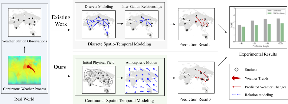
To address the above challenges, this paper introduces the Continuous Diffusive Prediction Network (CDPNet), which models atmospheric motion continuity from both spatial and temporal perspectives. The proposed model contains a Continuous Calibrated Initialization (CCI) module and a Diffusive Difference Estimation (DDE) module, respectively representing the continuous initial physical field and the evolving atmospheric process. Specifically, the CCI module begins by interpolating data between observation stations to create a coarse spatially continuous physical field. It then refines this field by incorporating densely predicted results from the previous time step and the global directional information of the overall trend. The previous time step's predictions enhance the temporal dependence, while the directional information ensures the continuity from a global perspective. After the precise continuous representation, the DDE module explicitly models the spatial diffusion process and estimates the diffusive difference between the current time step and the subsequent one. This approach, simulating the atmospheric motion process, effectively captures motion continuity both spatially and temporally, and reflects the variations at individual stations across time steps. Similarly, we also incorporate the directional information on weather changes from the entire historical sequence to mitigate the estimation uncertainty, thereby further constraining the temporal continuity and enhancing the weather prediction performance. Extensive experiments show that the proposed model outperforms existing state-of-the-art approaches on the Weather2K and Global Wind/Temp datasets. Especially on the Weather2K dataset, the proposed model can bring at least a 4.48% improvement in Mean Absolute Error (MAE) compared to other models.
In summary, the main contributions of this paper are as follows:
- We propose the CDPNet, which models the real-world continuous weather change process from discrete station observation data, enhancing the accuracy of weather prediction.
- We propose the CCI module to construct the initial physical field through spatial interpolation and directional information calibration. It accurately represents the current physical state and provides a foundation for future weather prediction.
- We propose the DDE module to explicitly model continuous atmospheric motion through spatial diffusion process and directional information correction. It infers the evolution of the physical field and accurately predicts the weather at the next time step.
- Extensive experiments show that the proposed model significantly outperforms existing state-of-the-art models. Especially on the Weather2K dataset, the proposed CDPNet can bring at least a 4.48% improvement in MAE compared to other models.
2 Methodology
Previous studies fail to accurately model the continuous physical process of atmospheric motion, resulting in unsatisfactory weather prediction results. Therefore, we propose a weather prediction model called the Continuous Diffusive Prediction Network (CDPNet) with a Continuous Calibrated Initialization (CCI) module and a Diffusive Difference Estimation (DDE) module.
2.1 Overall Architecture
Given the historical observations X1:L = {x1, x2, · · · , xL} ∈ RN×L×C (including N weather stations, C weather variables such as temperature and wind speed over the past L time steps) and auxiliary variables Xaux (including station coordinates and time information), the goal of multi-station weather prediction is to forecast the weather conditions for the future P time steps,
{ˆxL+1, ˆxL+2, · · · , ˆxL+P} = F({x1, x2, · · · , xL}), (1) where F is the mapping function to be learned, and ˆXL+1:L+P = {ˆxL+1, ˆxL+2, · · · , ˆxL+P} ∈ RN×P×C represents the predicted future weather conditions.
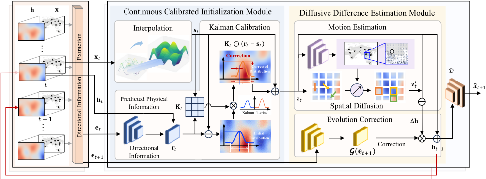
We propose the CDPNet which takes into account the continuous physical process of atmospheric motion to realize multi-station weather prediction. The network structure of CDPNet is based on Recurrent Neural Networks (RNN). For each time step t, the observation xt is input to the CDPNet to predict the weather ˆxt+1 at the next time step t + 1, and this process can be expressed as ˆxt+1 = FCDPNet(xt). Specifically, CDPNet contains two key modules: the CCI module FCCI and the DDE module FDDE. The CCI module is used to construct a continuous initial physical field zt, while the DDE module models the spatial diffusion process of atmospheric motion to predict the physical field ht+1 at the next time step. After obtaining the predicted physical field at the moment t + 1, we can map the physical field back to the station weather results ˆxt+1 by a convolutional decoder D. This process can be described as
The network architecture details of CDPNet is illustrated in Figure 2.
2.2 Continuous Calibrated Initialization (CCI) Module
Constructing an accurate continuous initialization of physical fields is challenging due to the sparse distribution of weather stations across large geographic areas. Therefore, the proposed Continuous Calibration Initialization module first coarsely models the continuous physical fields through the Inverse Distance Weighted (IDW) interpolation method [Shepard, 1968], and then calibrates the coarse representation by using the predicted physical field from the previous time step as well as the weather evolution direction information from the entire observational sequence.
Specifically, to model the spatial relations among sparse weather stations, we first project these stations onto a twodimensional grid representation based on their physical locations. Therefore, each grid could indicate the physical coordinates of a weather station, and display its observational data. For locations without actual weather stations, we use the widely-used IDW interpolation method to estimate the potential weather variable values. This process yields a coarse spatial continuous initialization of physical field st ∈ RH×W×C , where H and W are hyperparameters representing the dimensions of the physical field.
Distance-based interpolation of observational data cannot capture the spatial and temporal complexity of the weather systems. Therefore, we deploy the classical Kalman filter Kt to calibrate the coarse interpolation results. The Kalman filter is traditionally used for estimating the state of a linear dynamic system from a series of noisy measurements. It typically assumes that the system dynamics and measurement noise are both Gaussian and linear, though variations of the Kalman filter are used to handle non-linear systems. In this paper, we adopt a learnable convolution to approximate the non-linear Kalman filter, and consider both the predicted physical information ht derived from the previous time step and the current direction information et extracted from the entire history sequence as the measurements. Incorporating ht and et, rt could reflect the predicted continuous physical states of the current weather stations, and thus help capture the uncertainty related to the coarse interpolation. The learnable Kalman filter determines the weight given to rt in updating the coarse interpolation results. The calibrated process can be formulated as:
where || indicates the concatenate operation, σ, tanh are the sigmoid and hyperbolic tangent activation function, and fconv is the convolutional layer. wh, we and b are learnable parameters, to incorporate the predicted physical information ht and the direction information et.
The predicted physical field ht is derived from previous observational data xt-1, encompassing both predicted spatial and temporal continuity for current observations,
Incorporating ht also helps optimize the entire weather prediction model to generate accurate weather forecasting, thereby offering an informative representation for each time step.
For the direction information et, we adopt a multi-layer perceptron fMLP to capture the direction of the weather change at each moment from the entire historical sequence X1:L to constrain the temporal continuity:
where the auxiliary features Xaux can also be combined with historical observations, such as the latitude and longitude coordinates of the station and the time at each time step. We replicate Xaux to match the dimensions of the multistation historical observations X1:L ∈ RN×L×C to obtain Xaux 1:L ∈ RN×L×C .
Through the coarse spatial interpolation and the learnable Kalman calibration, the CCI module extracts comprehensive information from the observational data and constructs a spatio-temporally continuous initial physical field, which enhances the representation of current physical states and improves future weather predictions.
2.3 Diffusive Difference Estimation (DDE) Module
Accurately modeling the temporal evolution of the continuous physical field is highly challenging due to the differences in atmospheric motion across regions. To address this, the proposed DDE module predicts atmospheric motion directions at various locations and explicitly models the continuous spatial diffusion process, thereby enabling effective forecasting of future weather changes.
The constructed initial physical field takes into account the dense prediction results of the previous time step as well as the global directional information of the overall trend. Therefore, we can estimate the future atmospheric motion from the initial physical field. Specifically, we utilize a small convolutional neural network M to estimate the displacement [ui, uj ]
Algorithm 1 CDPNet training process
- Require: Training dataset T ; 1: while not converged do 2: Sample batch of sequences {X1:L,XL+1:L+P} ∼ T 3: Computing directional information from a global perspective {eL+1, eL+2, · · · , eL+P} = fMLP (cat [X1:L;Xaux 1:L ]) 4: for t ∈ [1, L + P ] do 5: // CCI Module 6: Spatial interpolation st = IDW(xt) 7: Construct the refined physical field rt = tanh (wh ∗ ht + we ∗ et + b) 8: Kalman calibration zt = st +Kt ⊙ (rt - st) 9: // DDE Module 10: Motion estimation ut =M(zt) 11: Calculating diffusive difference ∆h = z′t - zt 12: Predict the physical field for the next time step ht+1 = zt + G (et+1) ⊙ ∆h 13: // Decoding module 14: Decoding prediction results ˆxt+1 = D(ˆht+1) 15: end for 16: Update the model parameters based on the loss function L = ∥X1:L - ˆX1:L∥ + ∥XL+1:L+P - ˆXL+1:L+P ∥ 17: end while
of the atmospheric motion at any position [pi, pj] in continuous space from the initial physical field zt. This process can be expressed as [ui, uj ] = M(zt[pi, pj ]).
Based on the estimation of atmospheric motion, the spatial diffusion process between different geographical locations can be modeled. The diffusive difference ∆h can be expressed as:
where z′t denotes the diffused physical field. We consider the impact of atmospheric motion. For each geographical location [pi, pj] in the diffused physical field z′t , it is obtained by diffusing the initial physical field features zt from the location [pi -ui, pj -uj ]. The atmospheric motion displacement ui, uj are obtained from the motion estimation network M described above.
However, the diffusion process of a single time step is difficult to ensure the continuity of the weather change from a global perspective. Therefore, we consider inferring the direction information of the weather change at the current moment from the whole historical weather series to correct the diffusion difference. The complete diffusive difference estimation process can be written in the following form:
where ht+1 is the physical field at time step t + 1 estimated from the initial physical field zt. The G (·) is a simple convolutional network, and the direction information et+1 is computed in the same way as in Eq. (6).
Therefore, the DDE module considers the atmospheric motion and explicitly simulates the spatial diffusion process, while the weather change direction information extracted based on the whole historical sequence is used to constrain the time continuity and improve the weather prediction performance.
| Methods | Air Temperature | Relative Humidity | Wind Speed | Air Pressure | Avg. | |||||
|---|---|---|---|---|---|---|---|---|---|---|
| MAE | RMSE | MAE | RMSE | MAE | RMSE | MAE | RMSE | MAE | RMSE | |
| Autoformer | 1.7205 | 2.3498 | 9.6201 | 12.8131 | 0.9705 | 1.3365 | 1.4546 | 2.0618 | 3.4414 | 4.6403 |
| FEDformer | 1.6015 | 2.2255 | 8.1413 | 11.3160 | 0.9095 | 1.2782 | 1.1972 | 1.7509 | 2.9624 | 4.1427 |
| ASTGCN | 2.6942 | 3.6386 | 12.0332 | 15.9847 | 1.0130 | 1.4293 | 2.7041 | 3.6992 | 4.6111 | 6.1879 |
| MSTGCN | 3.6827 | 4.9195 | 14.4780 | 18.7188 | 0.9979 | 1.4102 | 2.8912 | 3.6243 | 5.5124 | 7.1682 |
| DCRNN | 5.0457 | 6.4070 | 16.3467 | 21.2517 | 0.8757 | 1.2514 | 1.9716 | 2.8879 | 6.0599 | 7.9495 |
| GCGRU | 1.8823 | 2.7491 | 7.7008 | 10.9422 | 0.8738 | 1.2424 | 1.8463 | 2.6466 | 3.0758 | 4.3951 |
| Corrformer | 1.8269 | 2.4493 | 9.0081 | 12.3344 | 0.9391 | 1.3226 | 2.1183 | 2.6525 | 3.4731 | 4.6897 |
| EasyST | 2.1142 | 2.7935 | 8.9515 | 12.0980 | 0.8672 | 1.2052 | 1.9149 | 2.5392 | 3.4620 | 4.6590 |
| PhyDNet | 1.6186 | 2.1265 | 7.8897 | 10.4605 | 0.9186 | 1.2883 | 1.8719 | 2.5740 | 3.0747 | 4.1123 |
| NowcastNet | 1.4544 | 1.9263 | 7.4994 | 10.0036 | 0.8868 | 1.2777 | 1.6216 | 2.2074 | 2.8656 | 3.8538 |
| CDPNet (Ours) | 1.3927 | 1.8576 | 7.2596 | 9.7500 | 0.8713 | 1.2334 | 1.4251 | 1.9771 | 2.7372 | 3.7045 |
| Factors | Metrics | Autoformer | FEDformer | DCRNN | Corrformer | EasyST | PhyDNet | NowcastNet | CDPNet (Ours) |
|---|---|---|---|---|---|---|---|---|---|
| Wind | MSE | 4.687 | 4.750 | 3.475 | 3.889 | 4.769 | 3.552 | 3.607 | 3.538 |
| MAE | 1.465 | 1.503 | 1.282 | 1.304 | 1.513 | 1.301 | 1.314 | 1.281 | |
| Temp | MSE | 10.142 | 11.054 | 8.401 | 7.709 | 9.177 | 7.234 | 7.495 | 6.949 |
| MAE | 2.250 | 2.405 | 1.941 | 1.888 | 2.213 | 1.895 | 1.931 | 1.843 | |
| Avg. | MSE | 7.415 | 7.902 | 5.938 | 5.799 | 6.973 | 5.393 | 5.551 | 5.244 |
| MAE | 1.858 | 1.954 | 1.612 | 1.596 | 1.863 | 1.598 | 1.623 | 1.562 |
papers, the data for training, validation, and testing are all one-year time. The task is set to predict 12 hours in the future based on the past 12 hours, where the input length is 12 steps and the prediction length is 12 steps.
Global Wind/Temp: It is from the National Centers for Environmental Information. This dataset contains the hourly averaged wind speed and hourly temperature of 3,850 stations around the world from January 1, 2019 to December 31, 2020. Like the setup in other papers, we split the dataset into training, validation, and test sets in chronological order by a ratio of 7:1:2. The task is set to predict one day in the future based on the past 2 days, where the input length is 48 steps and the prediction length is 24 steps.
Implementation details
Our model is implemented using PyTorch 2.1.0 and trained on an NVIDIA GeForce RTX 2080 Ti GPU. We employ the Adam optimizer with a batch size of 1 to accommodate the large number of stations in our dataset. The training process consists of two distinct phases: first, we initialize the direction information by training for one epoch with a learning rate of 0.001, followed by training the entire network with a reduced learning rate of 0.00001. The model undergoes training for up to 100 epochs, with an early stopping mechanism implemented to prevent overfitting. The implementation code is publicly available at https://github.com/ChujieXu/CDPNet.
Evaluation metrics
We measure our model and other methods by three common deviation-based evaluation metrics: Mean Squared Error (MSE), Mean Absolute Error (MAE), and Root Mean Squared Error (RMSE).
2.4 Optimization
The overall training flow is shown in Algorithm 1, and we use an iterative generation approach to predict the weather at the next time step based on the information at the current time step, which is consistent with the RNN architecture. Specifically, for historical moments, we reconstruct the entire historical sequence X1:L, this is to ensure that the evolution of the weather field is consistent with the variation of the real weather. For future moments, the model generates the final result ˆXL+1:L+P .
The optimization objective during training is two-fold: to minimize the reconstruction error of the historical sequence and the prediction error of the future sequence. This is formalized as follows:
where both parts of the loss are optimized using l1 loss.
3 Experiments
In this section, extensive experiments were conducted to validate the effectiveness of the proposed CDPNet.
3.1 Experimental Settings
Data description
In this paper, experiments are carried out on two real datasets, including the Weather2K dataset [Zhu et al., 2023] and the Global Wind/Temp dataset [Wu et al., 2023].
Weather2K: It covers 31 provinces in China and contains 1,866 ground weather stations. The time scale is from January 1, 2017 to December 31, 2019. Based on meteorological consideration, 20 important near-surface meteorological factors and 3 time-invariant constants for position information are provided in the Weather2K. Like the setup in other
| Air Temperature | Relative Humidity | Wind Speed | Air Pressure | Avg. | ||||||
|---|---|---|---|---|---|---|---|---|---|---|
| MAE | RMSE | MAE | RMSE | MAE | RMSE | MAE | RMSE | MAE | RMSE | |
| Baseline | 3.5391 | 4.5073 | 12.4065 | 15.4771 | 1.1013 | 1.5426 | 4.8061 | 6.2843 | 5.4633 | 6.9528 |
| + CCI Module | 1.4793 | 1.9506 | 7.8748 | 10.3929 | 0.8956 | 1.3515 | 1.5663 | 2.1602 | 2.9540 | 3.9638 |
| + DDEModule | 1.4635 | 1.9324 | 7.6587 | 10.1423 | 0.8751 | 1.2768 | 1.3796 | 1.9397 | 2.8442 | 3.8228 |
| CDPNet (Ours) | 1.3927 | 1.8576 | 7.2596 | 9.7500 | 0.8713 | 1.2334 | 1.4251 | 1.9771 | 2.7372 | 3.7045 |
3.2 Performance Comparison
To comprehensively demonstrate the effectiveness of the proposed CDPNet model, we compared it with various prediction models based on different motivations, which can be roughly classified into two categories: time series prediction models, such as Autoformer [Wu et al., 2021] and FEDformer [Zhou et al., 2022], focusing on the time dependence of meteorological variables at individual stations; and spatiotemporal predictive models, such as ASTGCN [Guo et al., 2019], MSTGCN [Guo et al., 2019], DCRNN [Li et al., 2018], GCGRU [Seo et al., 2018], Corrformer [Wu et al., 2023] and EasyST [Tang et al., 2024], which focus on spatial correlations between multiple stations. Additionally, we considered other methods incorporating physical information, such as PhyDNet [Guen and Thome, 2020] and NowcastNet [Zhang et al., 2023]. Based on the proposed CDPNet, we compared the key physical modules of these methods with our proposed DDE module.
As can be seen from Table 1, our model outperforms other comparison methods using both MAE and RMSE metrics on the Weather2K dataset, which indicates the superiority of CDPNet. For the four most common meteorological variables of air temperature, relative humidity, wind speed, and air pressure, CDPNet obtained an average MAE of 2.7372 and an average RMSE of 3.7045, which are 4.48% and 3.87% improvement compared to the suboptimal method, respectively. As shown in Table 2, we similarly validated on the Global Wind/Temp dataset with a wider range and a larger number of stations. From Table 2, we can see the performance gain is also evident, demonstrating the practicability of our model. For the two variables of temperature and wind speed, CDPNet obtained an average MSE of 5.244 and an average MAE of 1.562, which obtained the best performance.
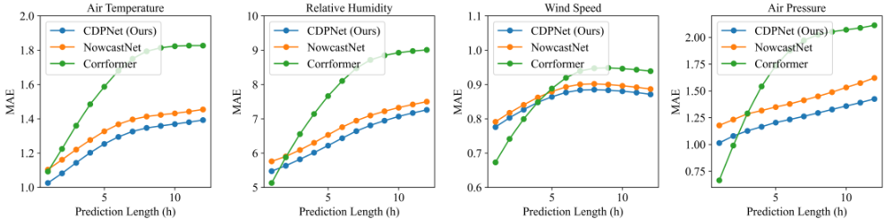
Besides the overall performance evaluation, we also compared the prediction errors across different forecasting lengths, as shown in Figure 3. The prediction errors of the proposed CDPNet consistently remain lower than that of NowcastNet. On the other hand, Corrformer achieves higher accuracy in the short term but experiences a sharp decline in performance as the forecasting length increases. This indicates that the proposed CDPNet is better at capturing longtermweather trends.
3.3 Ablation Study
In this section, we conduct ablation studies to analyze the effectiveness of the designed components in the proposed model. Table 3 outlines the findings of the baseline model, baseline model with the proposed CCI module, baseline model with the proposed DDE module, and baseline model with CCI module and DDE module (our CDPNet). The baseline model with CCI module means that this approach does not perform complex diffusive difference estimation. Instead, it uses a simple convolutional network to map the constructed initial physical field to future time steps for prediction. The baseline model with DDE module means that instead of performing continuous calibrated initialization, it employs simple reshaping and convolution operations to transform discrete stations into a two-dimensional space. As shown in Table 3, CCI module helps real-world modeling to predict weather conditions due to its ability to construct a continuous initial physical field. The MAE decreases from 5.4633 to 2.9540, and the RMSE decreases from 6.9528 to 3.9638. After adding the DDE module to estimate the atmospheric motion considering the weather evolution, a more significant performance improvement is observed. The MAE of the proposed model decreases from 5.4633 to 2.8442 and the RMSE decreases from 6.9528 to 3.8228. When both CCI module and DDE module are applied to the baseline model, the model structure is the same as the proposed CDPNet model. The model achieves an optimal MAE of 2.7372, as well as an optimal RMSE of 3.7045. All these results indicate that each component of our model contributes significantly to the final CDPNet model, resulting in the best performance.
3.4 Parameter Sensitivity
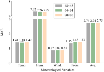
The core of the proposed CDPNet method lies in the initialization and diffusion of the physical field. Therefore, we conducted experiments to explore the impact of the physical field size on prediction performance. As shown in Figure 4, we compared the effects of the physical field sizes of 48×48, 64×64, and 80×80 on the final prediction performance. The experiments revealed that the size of the physical field had little overall impact on the results. This is because the physical field features already exhibit strong spatio-temporal continuity, and changes in resolution have a limited effect on extracting key information. Even at lower resolutions, the primary physical trends can still be captured effectively.
3.5 Visual Analysis
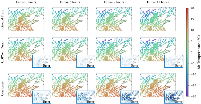
To validate the effectiveness of the proposed CDPNet method, we visualize the prediction results in a local area of northern China. As shown in Figure 5, a comparison is presented between the temperature predictions of CDPNet (our model) and Corrformer (comparison method) with the ground truth for the next 3, 6, 9, and 12 hours. Each row represents a different model, and each column corresponds to the predictions at different times. Redder colors indicate higher temperatures, with the color bar on the right displaying the temperature range. Additionally, there are error maps below the predictions of CDPNet and Corrformer, where color intensity reflects the prediction error, allowing for a visual comparison of each model's accuracy at different times. The figure reveals that CDPNet has smaller errors in temperature predictions for the next 3, 6, 9, and 12 hours, with wider low-error regions. In contrast, Corrformer has larger errors, particularly at 9 and 12 hours. This indicates that CDPNet, through continuous modeling, effectively captures the spatiotemporal dependencies of temperature variations, enabling it to more accurately reflect the dynamic temperature changes, thus achieving higher prediction accuracy across different periods.
4 Conclusion
In this paper, the CDPNet is proposed to improve the accuracy of multi-station weather prediction by capturing the continuity of atmospheric motions in both space and time. CDPNet simulates the initial physical field and the atmospheric diffusion process of the weather station through the CCI module and the DDE module. Experimental results show that CDPNet can effectively capture the continuity of atmospheric motion in space and time, and outperforms previous deep learning methods on multiple datasets. In particular, on the Weather2K dataset, CDPNet demonstrates a significant advantage in terms of MAE.
Acknowledgments
This work was supported by National Natural Science Foundation of China under Grant 62476018.
@inproceedings{ijcai2025p747,
  title     = {Continuous Diffusive Prediction Network for Multi-Station Weather Prediction},
  author    = {Xu, Chujie and Ma, Yuqing and Deng, Haoyuan and Gao, Yajun and Wang, Yudie and Lv, Kai and Liu, Xianglong},
  booktitle = {Proceedings of the Thirty-Fourth International Joint Conference on
               Artificial Intelligence, {IJCAI-25}},
  publisher = {International Joint Conferences on Artificial Intelligence Organization},
  editor    = {James Kwok},
  pages     = {6714--6722},
  year      = {2025},
  month     = {8},
  note      = {Main Track},
  doi       = {10.24963/ijcai.2025/747},
  url       = {https://doi.org/10.24963/ijcai.2025/747},
}
TY - CPAPER TI - Continuous Diffusive Prediction Network for Multi-Station Weather Prediction AU - Xu, Chujie AU - Ma, Yuqing AU - Deng, Haoyuan AU - Gao, Yajun AU - Wang, Yudie AU - Lv, Kai AU - Liu, Xianglong T2 - Proceedings of the Thirty-Fourth International Joint Conference on Artificial Intelligence, IJCAI-25 PB - International Joint Conferences on Artificial Intelligence Organization PY - 2025 SP - 6714 EP - 6722 DO - 10.24963/ijcai.2025/747 UR - https://doi.org/10.24963/ijcai.2025/747 ER -Copied
Machine-readable versions of this paper, for tools and AI agents:





